计算机视觉3.1：数据增强

最新推荐文章于 2024-04-08 08:30:00 发布

俯仰天地

最新推荐文章于 2024-04-08 08:30:00 发布

阅读量3.1k

点赞数 1

分类专栏：计算机视觉文章标签：计算机视觉机器学习深度学习

本文链接：https://blog.csdn.net/weixin_43669978/article/details/121160489

版权

计算机视觉专栏收录该内容

20 篇文章 2 订阅

订阅专栏

数据增强

Any modification we make to a learning algothrithm that is intended to reduce its generalization error but not its training error.

——Goodfellow et.al

我们对（深度）学习算法所做的所有调整都是为了减少其泛化误差，而非训练误差。

我们之前所说的正则方法，正是通过以增大训练误差为代价来减少泛化误差的。

我们之前所提到的正则方法都是以参数化的形式出现的，需要去更新权重、loss等，实际上，还存在着其他形式的正则方法。

网络自己调整自己的网络结构（Dropout）
增加传递进网络用于训练的数据。

在接下来的篇幅中，我们将会讨论第2中类型的正则，称之为数据增强。这种方法有意干扰训练样本，在将其传入神经网络之前轻微改变其外表。这样做会导致一个神经网络不断的“看见“新的数据，这些新的数据都是从训练数据中生成的，部分减轻了我们升级数据的压力。

什么是数据增强？

数据增强包含广泛的一些系列用于通过抖动和干扰从原始样本生成新的训练样本，但是类标签不改变的技术。

进行数据增强的目的是为了增加模型的泛化能力。 假如我们所要训练的网络不断的看到新的，轻微变动的输入样本点，那么它就能学到更加健壮的特征。

而在测试是，我们不用数据增强，所以在大多数情况下，测试准确率会有所上升，但是以训练准确度的轻微下降为代价。

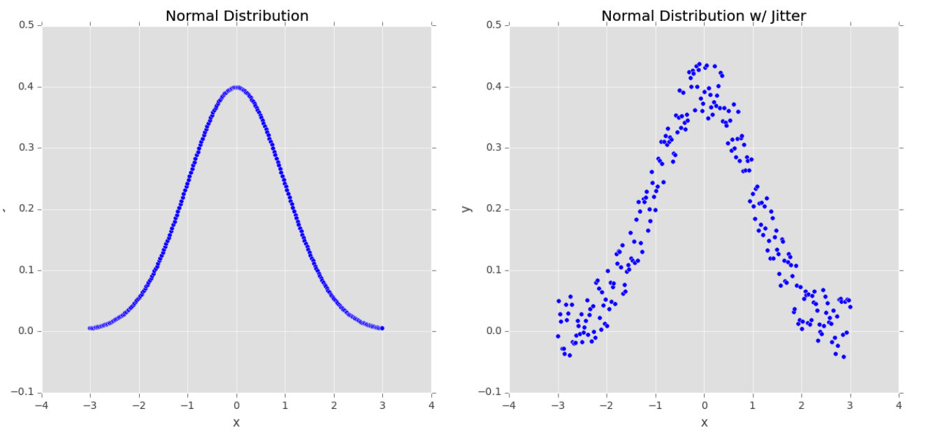
我们来分析一下上面这张图（本文图片皆引用自：Deep Learning for Computer Version with Python），左边是平均值为0的正态分布，在此数据上训练机器学习模型也许会准确的将此模型刻画出来，但在现实世界中，数据很少服从如此整齐的分布。

相反，为了提高分类器的泛化能力，我们也许会先通过给沿着分布曲线的样本点随机加上一些 $\varepsilon$ 值来生成随机的抖动样本点，如右图所示。我们的数据依然服从近似的正态分布，，但它不再像左图一样是一个完美的正态分布，在此数据上训练出来的模型对于不在数据集之外的数据所表现出来的泛化能力更好一些。

我们可以通过对图像进行简单的集合变化来获得额外的训练数据，包括随机的：

平移
旋转
缩放
修剪
水平翻转、垂直翻转（有时会改变标签类别）

对于计算机视觉方向来说更加高级的数据增强技术还包括对给定色彩空间进行随机的干扰，和非线性几何扭曲。

数据增强可视化

理解数据增强的最好的方法就是对增强过的图片进行简单的可视化。我们可以创建名augmentation_demo.py的脚本文件，写入如下代码

from tensorflow.keras.preprocessing.image import ImageDataGenerator
from tensorflow.keras.preprocessing.image import img_to_array
from tensorflow.keras.preprocessing.image import load_img
import numpy as np

# 原始图像存储路径
image = r"E:\PycharmProjects\DLstudy\practice-bundle\1.png"
# 增强后的图像的输出路径
output = r"E:\PycharmProjects\DLstudy\practice-bundle\augmented_result"
# 输出的图像的前缀名
prefix = "image"

# 加载样本图片
print("[INFO] loading example image...")
image = load_img(image)
image = img_to_array(image)
image = np.expand_dims(image, axis=0)

# 创建图像数据生成器
aug = ImageDataGenerator(rotation_range=30,  width_shift_range=0.1, height_shift_range=0.1, shear_range=0.2,
                         zoom_range=0.5, horizontal_flip=True, fill_mode="nearest")
total = 0

# 用图像数据生成器生出图像
print("[INFO] generating images...")
imageGen = aug.flow(image, batch_size=1, save_to_dir=output,
                    save_prefix=prefix, save_format="jpg")

# 控制生成的图像的数量
for image in imageGen:
    total += 1

    if total == 10:
        break

运行结果

可以看到这些图片是在原图的基础上进行了随机的平移、旋转、修剪、缩放、翻转等操作。

但是，我们接下来会发现：数据增强有助于大幅度降低过拟合程度。

当用包含很少样本的数据集来训练深度学习时，我们可以利用数据增强技术来产生额外的训练数据，借此来减少手工标注数据的数量。

对比有无数据增强的训练结果

对于数据增强技术，我们要进行两个实验：

不用数据增强技术，在Flower-17数据集上训练MiniVGGNet
用数据增强技术，在Flower-17数据集上训练MiniVGGNet

我们将会发现，使用数据增强会大幅度降低过拟合程度，并让MiniVGGNet获得更高的在准确率。

Flower-17数据集

详细介绍点击：Flower-17数据集

图像预处理

到目前为止，我们都是通过将图像大小改变为一个固定的尺寸来预处理图像，并未考虑纵横比。在某些情况下，尤其是基准数据集，这样做是可取的。

但是，对于大多数具有挑战性的数据集我们仍然会将其大小改变到一个固定的尺寸，但是会保持其纵横比。下图说明了这个过程。

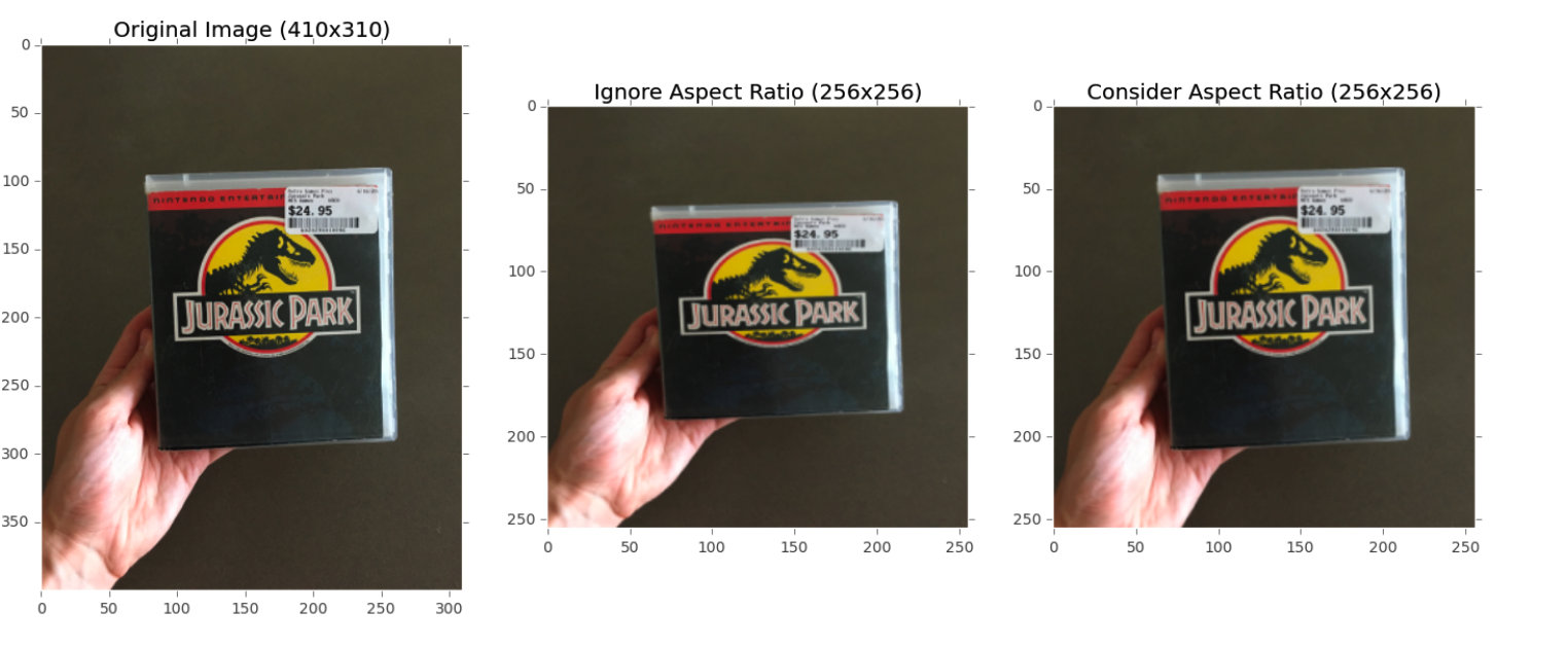
上图中，最左边是原始图像，中间是改变大小但未保持横纵比，右边同样改变了大小但保持了横纵比。

当我们有效地丢弃了部分图像时，我们同样也保持了图像的横纵比。

保持一致的横纵比可以使得我们的卷积神经网络学到更加细微、一致的特征。

让我们一起实现这个预处理的过程吧：

目录结构如下：

----pyimgsearch
|		|----__init__.py
|		|----callbacks		
|		|----nn
|		|preprocessing
|		|		|__init__.py
|		|		|----aspectawarepreprocessor.py
|		|		|----imagetoarraypreprocessor.py
|		|		|----simplepreprocessor.py
|		|----utils

打开aspectawarepreprocessor.py，写入如下代码

import imutils
import cv2


class AspectAwarePreprocessor:
    def __init__(self, width, height, inter=cv2.INTER_AREA):
        self.width = width
        self.height = height
        self.inter = inter

    def preprocess(self, image):
        (h, w) = image.shape[:2]
        dW = 0
        dH = 0

        if w < h:
            image = imutils.resize(image, width=self.width, inter=self.inter)
            dH = int((image.shape[0] - self.height) / 2.0)
        else:
            image = imutils.resize(image, height=self.height, inter=self.inter)
            dW = int((image.shape[1] - self.width) / 2.0)

        (h, w) = image.shape[:2]
        image = image[dH:h - dH, dW:w - dW]

        return cv2.resize(image, (self.width, self.height), interpolation=self.inter)

接下来让我们将其用于训练MiniVGGNet结构。

MiniVGGNet on Flower-17：无数据增强

创建minivggnet_flower17.py，写入如下代码

from sklearn.preprocessing import LabelBinarizer
from sklearn.model_selection import train_test_split
from sklearn.metrics import classification_report
from pyimagesearch.preprocessing.aspepctawarepreprocessor import AspectAwarePreprocessor
from pyimagesearch.preprocessing.imagetoarraypreprocessor import ImageToArrayPreprocessor
from pyimagesearch.datasets.simpledatasetsloader import SimpleDatasetLoader
from nn.conv.minivggnet import MiniVGGNet
from tensorflow.keras.optimizers import SGD
from imutils import paths
import matplotlib.pyplot as plt
import numpy as np
import os

# 定义训练集的存放路径
dataset = "/Users/liushanlin/Desktop/数据集/Flower17-master/dataset/train"

# 加载训练图像并根据路径名提取类别标签
print("[INFO] loading images...")
imagePaths = list(paths.list_images(dataset))
classNames = [pt.split(os.path.sep)[-2] for pt in imagePaths]
classNames = [str(x) for x in np.unique(classNames)]

# 预处理图像
aap = AspectAwarePreprocessor(64, 64)
iap = ImageToArrayPreprocessor()
sdl = SimpleDatasetLoader(preprocessor=[aap, iap])
(data, labels) = sdl.load(imagePaths, verbose=500)
data = data.astype("float") / 255.0

# 分割数据集 
(trainX, testX, trainY, testY) = train_test_split(data, labels, test_size=0.25, random_state=42)
trainY = LabelBinarizer().fit_transform(trainY)
testY = LabelBinarizer().fit_transform(testY)

# 编译模型
print("[INFO] compiling model...")
opt = SGD(learning_rate=0.05)
model = MiniVGGNet.build(width=64, height=64, depth=3, classes=len(classNames))
model.compile(loss="categorical_crossentropy", optimizer=opt, metrics=["accuracy"])

# 训练模型
print("[INFO] training network")
H = model.fit(trainX, trainY, validation_data=(testX,testY), batch_size=32, epochs=100, verbose=1)

# 评估模型并输出评价报告
print("[INFO] evaluating network...")
predictions = model.predict(testX, batch_size=32)
print(classification_report(testY.argmax(axis=1), predictions.argmax(axis=1), target_names=classNames))

#绘图 
plt.style.use("ggplot")
plt.figure()
plt.plot(np.arange(0, 100), H.history["loss"], label="train_loss")
plt.plot(np.arange(0, 100), H.history["val_loss"], label="val_loss")
plt.plot(np.arange(0, 100), H.history["accuracy"], label="train_acc")
plt.plot(np.arange(0, 100), H.history["val_accuracy"], label="val_acc")
plt.savefig("/Users/liushanlin/PycharmProjects/DLstudy/result/MiniVGGNet_On_Cifar10.png")

执行结果：

              precision    recall  f1-score   support

    bluebell       1.00      0.94      0.97        31
   buttercup       1.00      0.89      0.94        37
  colts_foot       0.93      0.88      0.90        32
     cowslip       0.85      0.85      0.85        40
      crocus       0.89      1.00      0.94        33
    daffodil       0.93      0.93      0.93        30
       daisy       0.84      1.00      0.91        42
   dandelion       0.89      0.94      0.91        34
  fritillary       0.94      1.00      0.97        31
        iris       1.00      0.82      0.90        34
 lily_valley       0.85      0.94      0.89        35
       pansy       0.87      0.93      0.90        29
    snowdrop       0.94      0.94      0.94        36
   sunflower       0.95      1.00      0.97        36
   tigerlily       1.00      0.71      0.83        34
       tulip       0.72      0.95      0.82        38
  windflower       1.00      0.72      0.84        43

    accuracy                           0.91       595
   macro avg       0.92      0.91      0.91       595
weighted avg       0.92      0.91      0.91       595

MiniVGGNet on Flower-17：数据增强

创建miniVGGNet_on_flower17_Data.py脚本，写入如下代码：

from sklearn.preprocessing import LabelBinarizer
from sklearn.model_selection import train_test_split
from sklearn.metrics import classification_report
from pyimagesearch.preprocessing.aspepctawarepreprocessor import AspectAwarePreprocessor
from pyimagesearch.preprocessing.imagetoarraypreprocessor import ImageToArrayPreprocessor
from pyimagesearch.datasets.simpledatasetsloader import SimpleDatasetLoader
from nn.conv.minivggnet import MiniVGGNet
from tensorflow.keras.preprocessing.image import ImageDataGenerator
from tensorflow.keras.optimizers import SGD
from imutils import paths
import matplotlib.pyplot as plt
import numpy as np
import os

# 定义训练集的存放路径
dataset = "/Users/liushanlin/Desktop/数据集/Flower17-master/dataset/train"

# 加载训练图像并根据路径名提取类别标签
print("[INFO] loading images...")
imagePaths = list(paths.list_images(dataset))
classNames = [pt.split(os.path.sep)[-2] for pt in imagePaths]
classNames = [str(x) for x in np.unique(classNames)]

# 预处理图像
aap = AspectAwarePreprocessor(64, 64)
iap = ImageToArrayPreprocessor()
sdl = SimpleDatasetLoader(preprocessor=[aap, iap])
(data, labels) = sdl.load(imagePaths, verbose=500)
data = data.astype("float") / 255.0

# 分割数据集
(trainX, testX, trainY, testY) = train_test_split(data, labels, test_size=0.25, random_state=42)
trainY = LabelBinarizer().fit_transform(trainY)
testY = LabelBinarizer().fit_transform(testY)

#  构建其用于数据增强的图像生成器
aug = ImageDataGenerator(rotation_range=30, width_shift_range=0.1, height_shift_range=0.1,
                         shear_range=0.2, zoom_range=0.2, horizontal_flip=True, fill_mode="nearest")

# 编译模型
print("[INFO] compiling model...")
opt = SGD(learning_rate=0.05)
model = MiniVGGNet.build(width=64, height=64, depth=3, classes=len(classNames))
model.compile(loss="categorical_crossentropy", optimizer=opt, metrics=["accuracy"])

# 训练模型
print("[INFO] training network")
H = model.fit(aug.flow(trainX, trainY, batch_size=32), validation_data=(testX, testY),
              steps_per_epoch=len(trainX) // 32, epochs=100, verbose=1)

# 评估模型并输出评价报告
print("[INFO] evaluating network...")
predictions = model.predict(testX, batch_size=32)
print(classification_report(testY.argmax(axis=1), predictions.argmax(axis=1), target_names=classNames))

#绘图
plt.style.use("ggplot")
plt.figure()
plt.plot(np.arange(0, 100), H.history["loss"], label="train_loss")
plt.plot(np.arange(0, 100), H.history["val_loss"], label="val_loss")
plt.plot(np.arange(0, 100), H.history["accuracy"], label="train_acc")
plt.plot(np.arange(0, 100), H.history["val_accuracy"], label="val_acc")
plt.title("Training Loss and Accuracy with Data Augmentation")
plt.xlabel("Epoch#")
plt.ylabel("Loss/Accuracy")
plt.legend()
plt.savefig("/Users/liushanlin/PycharmProjects/DLstudy/result/MiniVGGNet_On_Cifar10_DataAug.png")

运行结果：

              precision    recall  f1-score   support

    bluebell       1.00      0.97      0.98        31
   buttercup       1.00      0.86      0.93        37
  colts_foot       0.75      0.94      0.83        32
     cowslip       0.90      0.90      0.90        40
      crocus       0.73      1.00      0.85        33
    daffodil       1.00      0.77      0.87        30
       daisy       1.00      0.98      0.99        42
   dandelion       0.97      1.00      0.99        34
  fritillary       0.84      1.00      0.91        31
        iris       1.00      0.82      0.90        34
 lily_valley       0.95      1.00      0.97        35
       pansy       1.00      0.93      0.96        29
    snowdrop       0.94      0.92      0.93        36
   sunflower       0.95      0.97      0.96        36
   tigerlily       1.00      0.94      0.97        34
       tulip       0.90      0.95      0.92        38
  windflower       1.00      0.84      0.91        43

    accuracy                           0.93       595
   macro avg       0.94      0.93      0.93       595
weighted avg       0.94      0.93      0.93       595

俯仰天地

关注

1
点赞
踩
6

收藏

觉得还不错? 一键收藏
1
评论
计算机视觉3.1：数据增强

数据增强Any modification we make to a learning algothrithm that is intended to reduce its generalization error but not its training error. ——Goodfellow et.al我们对（深度）学习算法所做的所有调整都是为了减少其泛化误差，而非训练误差。我们之前所说的正则方法，正是通过以增大训练误差为代价来减
复制链接

扫一扫