


文章目录
一、MINISUT-model-build-infer(官方提供的sample)
1)类和对应函数介绍
- SampleOnnxMNIST类的作用
是一个用于处理 ONNX 模型的 TensorRT 示例类。它包含了构建引擎、执行推理以及处理输入和输出数据的功能 - 参数解释
    ①samplesCommon::OnnxSampleParams mParams;
    ②nvinfer1::Dims                  mInputDims;
    ③nvinfer1::Dims                  mOutputDims;
    ④int mNumber{0};

    /* 使用智能指针来指向引擎,方便生命周期管理 */
    ⑤std::shared_ptr<nvinfer1::ICudaEngine> mEngine;
①mParam的作用
类型为 samplesCommon::OnnxSampleParams,用于存储构建和推理所需的参数。这个变量在构造函数中被初始化,并且在类的其他方法中被使用,例如 build 和 infer。
②mEngine的作用
类型为 std::shared_ptrnvinfer1::ICudaEngine,用于存储 TensorRT 引擎。这个变量在 build 方法中被初始化,并且在 infer 方法中被使用
③mInputDims的作用
类型为 nvinfer1::Dims,用于存储输入数据的维度信息。这个变量在 build 方法中被初始化,并且在 infer 方法中被使用
④mOutputDims的作用
类型为 nvinfer1::Dims,用于存储输出数据的维度信息。这个变量在 build 方法中被初始化,并且在 infer 方法中被使用
- 接口函数作用
①构造函数
    SampleOnnxMNIST(const samplesCommon::OnnxSampleParams& params)
        : mParams(params)
        , mEngine(nullptr)
    {
    }
②创建网络
    bool constructNetwork(
        SampleUniquePtr<nvinfer1::IBuilder>& builder,
        SampleUniquePtr<nvinfer1::INetworkDefinition>& network,
        SampleUniquePtr<nvinfer1::IBuilderConfig>& config,
        SampleUniquePtr<nvonnxparser::IParser>& parser);
③处理输入数据
    bool processInput(const samplesCommon::BufferManager& buffers);
④验证输出数据
    bool verifyOutput(const samplesCommon::BufferManager& buffers);
 ⑤构建模型引擎
     bool build();
 ⑥进行模型推理
    bool infer();
①构造函数
1>初始化类的实例,并传入一个 OnnxSampleParams 对象,该对象包含了构建和推理所需的参数。
2>初始化成员变量 mParams 为传入的参数,mEngine 初始化为 nullptr
②构建网络
1>构建 TensorRT 引擎。
2>该方法创建一个 IBuilder 对象、一个 INetworkDefinition 对象和一个 IBuilderConfig 对象。
3>使用 nvonnxparser::IParser 对象将 ONNX 模型解析并构建为 TensorRT 网络。
4>配置并序列化引擎,最终将引擎存储在 mEngine 成员变量中。
③处理输入数据
1>bool processInput(const samplesCommon::BufferManager& buffers):
2>处理输入数据。该方法将输入数据从 BufferManager 中读取,并进行必要的预处理。
3>MNIST前处理的实现:①读取随机digit数据;②分配buffers中的host上的空间;③将数据转为浮点数
④验证输出数据
1>bool verifyOutput(const samplesCommon::BufferManager& buffers):
2>验证输出数据。该方法将推理结果与预期输出进行比较,以验证推理的正确性。
3>MNIST后处理的实现:①分配输出所需要的空间;②手动实现一个cpu版本的softmax;③输出最大值以及所对应的digit class;
⑤创建网络build
 * 创建网络的流程基本上是这样:
 * 1. 创建一个builder
 * 2. 通过builder创建一个network
 * 3. 通过builder创建一个config
 * 4. 通过config创建一个opt(这个案例中没有)
 * 5. 对network进行创建
 *      - 可以使用parser直接将onnx中各个layer转换为trt能够识别的layer (这个案例中使用的是这个)
 *      - 也可以通过trt提供的ILayer相关的API自己从零搭建network (后面会讲)
 * 6. 序列化引擎(这个案例中没有)
 * 7. Free(如果使用的是智能指针的话,可以省去这一步)
2)整体流程
1、main函数中读取环境变量作为参数
    samplesCommon::Args args;
    bool argsOK = samplesCommon::parseArgs(args, argc, argv);
2、创建logger来保存日志(日志一般都是继承nvinfer1::ILogger来实现一个自定义的)
    auto sampleTest = sample::gLogger.defineTest(gSampleName, argc, argv);
    sample::gLogger.reportTestStart(sampleTest);
3、创建tensorRT示范类,用于解析onnx模型、构建模型和推理
SampleOnnxMNIST sample(initializeSampleParams(args));
4、创建推理模型
    if (!sample.build())
    {
        return sample::gLogger.reportFail(sampleTest);
    }
5、推理
    if (!sample.infer())
    {
        return sample::gLogger.reportFail(sampleTest);
    }
3)编译步骤
1、进入到TensorRT安装的目录
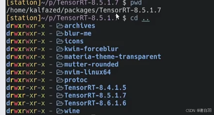
2、选择进入的TensorRT版本,并进入samples目录
#假如今天使用8.6.1.6版本
cd TensorRT-8.6.1.6
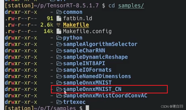
cd samples
3、把项目文件拷贝到这个samples目录
4、开始构建
make clean
make
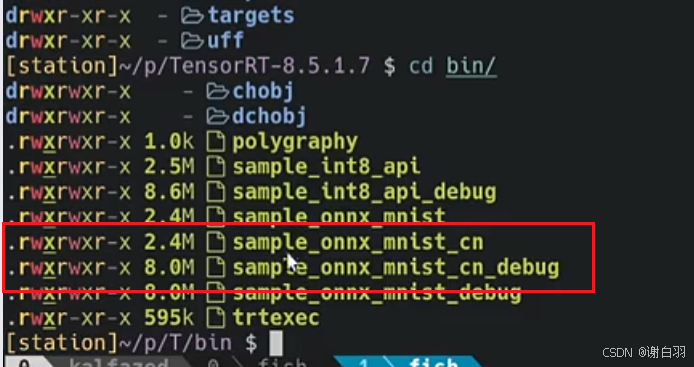
5、跳转出来到bin目录找到执行文件
cd ..
cd bin
4)更详细的代码讲解
(1)build构建网络流程
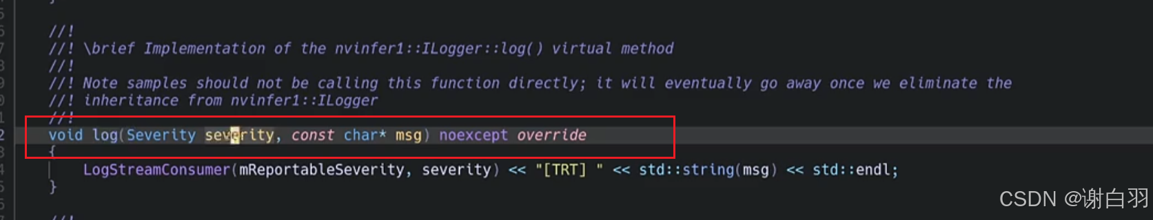
1、tensorRT在创建一个引擎的时候,需要绑定一个logger来打印日志,需要自己去实现虚函数log
2、构建网络builder的时候需要创建智能指针
    auto builder = SampleUniquePtr<nvinfer1::IBuilder>(nvinfer1::createInferBuilder(sample::gLogger.getTRTLogger()));
    if (!builder)
    {
        return false;
    }
SampleUniquePtr的实现(一个模板)
struct InferDeleter  //销毁obj
{
	template<typename T>
	void operator()(T* obj) const
	{
		delete obj;
	}
};

template <typename T>
using SampleUniquePtr = std::unique_ptr<T,InferDeleter>;
static auto StreamDeleter = [](cudaStream_t* pStream)
{
	if(pStream)
	{
		cudaStreamDestroy(*pStream);
		delete pStream;
	}
};
3、builder创建网络的时候用指针指针指向这个网络
    auto network = SampleUniquePtr<nvinfer1::INetworkDefinition>(builder->createNetworkV2(explicitBatch));
    if (!network)
    {
        return false;
    }
4、build的时候用builder创建一个config,也是用智能指针,同样的也是用parser从onnx中导出到network
    auto config = SampleUniquePtr<nvinfer1::IBuilderConfig>(builder->createBuilderConfig());
    if (!config)
    {
        return false;
    }
	//-----------------
    auto parser
        = SampleUniquePtr<nvonnxparser::IParser>(nvonnxparser::createParser(*network, sample::gLogger.getTRTLogger()));
    if (!parser)
    {
        return false;
    }
5、build的时候为网络配好配置,以及配好parser
备注:创建network的过程,如果不是用parser,需要自己一层一层的搭建,但这里是用parser一步到位
    auto constructed = constructNetwork(builder, network, config, parser);
    if (!constructed)
    {
        return false;
    }

bool SampleOnnxMNIST::constructNetwork(
    SampleUniquePtr<nvinfer1::IBuilder>& builder,
    SampleUniquePtr<nvinfer1::INetworkDefinition>& network,
    SampleUniquePtr<nvinfer1::IBuilderConfig>& config,
    SampleUniquePtr<nvonnxparser::IParser>& parser)
{
    auto parsed = parser->parseFromFile(locateFile(mParams.onnxFileName, mParams.dataDirs).c_str(),
        static_cast<int>(sample::gLogger.getReportableSeverity()));
    if (!parsed)
    {
        return false;
    }

    if (mParams.fp16)
    {
        config->setFlag(BuilderFlag::kFP16);
    }
    if (mParams.int8)
    {
        config->setFlag(BuilderFlag::kINT8);
        samplesCommon::setAllDynamicRanges(network.get(), 127.0f, 127.0f);
    }

    samplesCommon::enableDLA(builder.get(), config.get(), mParams.dlaCore);

    return true;
}
6、给profile设置cuda stream
不设置就会
1、失去对操作的精准控制
1)并行性受限
2)资源利用不充分
2、难以分析和调试程序性能
1)性能瓶颈难以定位:如果不设置cuda stream,程序的执行顺序和时间线会变得混乱,难以确定哪些操作时性能关键制约因素。设置后
可以将程序不同部分划分到不同流中,便于分析每个部分的执行时间和资源消耗,从而更准确的定位性能瓶颈
2)错误排查困难:不设置无法确定操作的执行顺序和相互的以来关系,判断不出错误是哪个操作或阶段产生
3、缺乏对程序执行的灵活性和可扩展性
1)难以适应不同硬件环境,不能充分发挥硬件的性能优势
2)难以扩展到多GPU或分布式计算环境
7、把network反序列化到engine里面
(2)infer推理
1、创建buffer
备注:bufferManger在创建时候就把host/device memory已经分配好了,否则需要自己计算engine的input输入/output输出的维度和大小,以及根据这些维度和大小进行malloc或者cudaMalloc内存分配
samplesCommon::BufferManager buffers(mEngine);
2、从engine创建一个context用来做推理
    samplesCommon::BufferManager buffers(mEngine);
    auto context = SampleUniquePtr<nvinfer1::IExecutionContext>(mEngine->createExecutionContext());
    if (!context)
    {
        return false;
    }
3、把数据进行前处理,并把数据拷贝到GPU设备上,并推理
    // 对于MNIST数据的preprocess(预处理)部分, 这个案例是在CPU上实现的
    ASSERT(mParams.inputTensorNames.size() == 1);
    if (!processInput(buffers))
    {
        return false;
    }

    // 将host上预处理好的数据copy到device上
    buffers.copyInputToDevice();
- 补充(前处理)
①读取随机digit数据
②分配buffers中的host上的空间
③将数据转为浮点数
bool SampleOnnxMNIST::processInput(const samplesCommon::BufferManager& buffers)
{
    const int inputH = mInputDims.d[2];
    const int inputW = mInputDims.d[3];

    // Read a random digit file
    srand(unsigned(time(nullptr)));
    std::vector<uint8_t> fileData(inputH * inputW);
    mNumber = rand() % 10;
    readPGMFile(locateFile(std::to_string(mNumber) + ".pgm", mParams.dataDirs), fileData.data(), inputH, inputW);

    // Print an ascii representation
    sample::gLogInfo << "Input:" << std::endl;
    for (int i = 0; i < inputH * inputW; i++)
    {
        sample::gLogInfo << (" .:-=+*#%@"[fileData[i] / 26]) << (((i + 1) % inputW) ? "" : "\n");
    }
    sample::gLogInfo << std::endl;

    float* hostDataBuffer = static_cast<float*>(buffers.getHostBuffer(mParams.inputTensorNames[0]));
    for (int i = 0; i < inputH * inputW; i++)
    {
        hostDataBuffer[i] = 1.0 - float(fileData[i] / 255.0);
    }

    return true;
}
4、把数据做后处理
①分配输出所需要空间
②手动实现一个cpu的softmax(softmax:将一个向量转换为表示各个类别相对概率的概率分布向量)
③输出最大值以及所对应的digit class
bool SampleOnnxMNIST::processInput(const samplesCommon::BufferManager& buffers)
{
    const int inputH = mInputDims.d[2];
    const int inputW = mInputDims.d[3];

    // Read a random digit file
    srand(unsigned(time(nullptr)));
    std::vector<uint8_t> fileData(inputH * inputW);
    mNumber = rand() % 10;
    readPGMFile(locateFile(std::to_string(mNumber) + ".pgm", mParams.dataDirs), fileData.data(), inputH, inputW);

    // Print an ascii representation
    sample::gLogInfo << "Input:" << std::endl;
    for (int i = 0; i < inputH * inputW; i++)
    {
        sample::gLogInfo << (" .:-=+*#%@"[fileData[i] / 26]) << (((i + 1) % inputW) ? "" : "\n");
    }
    sample::gLogInfo << std::endl;

    float* hostDataBuffer = static_cast<float*>(buffers.getHostBuffer(mParams.inputTensorNames[0]));
    for (int i = 0; i < inputH * inputW; i++)
    {
        hostDataBuffer[i] = 1.0 - float(fileData[i] / 255.0);
    }

    return true;
}
5)对应代码
- 代码
#include "argsParser.h"
#include "buffers.h"
#include "common.h"
#include "logger.h"
#include "parserOnnxConfig.h"
#include "NvInfer.h"
#include <cuda_runtime_api.h>
#include <cstdlib>
#include <fstream>
#include <iostream>
#include <sstream>
using namespace nvinfer1;
using samplesCommon::SampleUniquePtr;
const std::string gSampleName = "TensorRT.sample_onnx_mnist_cn";
/*
* 整个案例被封装到一个类里面了, 在类里面调用创建引擎和推理的实现
* 这个类实现了实现的隐蔽,用户通过这个类只能调用跟推理相关的函数build, infer
*/
class SampleOnnxMNIST
{
public:
SampleOnnxMNIST(const samplesCommon::OnnxSampleParams& params)
: mParams(params)
, mEngine(nullptr)
{
}
bool build();
bool infer();
private:
samplesCommon::OnnxSampleParams mParams;
nvinfer1::Dims mInputDims;
nvinfer1::Dims mOutputDims;
int mNumber{0};
/* 使用智能指针来指向引擎,方便生命周期管理 */
std::shared_ptr<nvinfer1::ICudaEngine> mEngine;
/* 创建网络 */
bool constructNetwork(
SampleUniquePtr<nvinfer1::IBuilder>& builder,
SampleUniquePtr<nvinfer1::INetworkDefinition>& network,
SampleUniquePtr<nvinfer1::IBuilderConfig>& config,
SampleUniquePtr<nvonnxparser::IParser>& parser);
bool processInput(const samplesCommon::BufferManager& buffers);
bool verifyOutput(const samplesCommon::BufferManager& buffers);
};
/*
* 创建网络的流程基本上是这样:
* 1. 创建一个builder
* 2. 通过builder创建一个network
* 3. 通过builder创建一个config
* 4. 通过config创建一个opt(这个案例中没有)
* 5. 对network进行创建
* - 可以使用parser直接将onnx中各个layer转换为trt能够识别的layer (这个案例中使用的是这个)
* - 也可以通过trt提供的ILayer相关的API自己从零搭建network (后面会讲)
* 6. 序列化引擎(这个案例中没有)
* 7. Free(如果使用的是智能指针的话,可以省去这一步)
*/
bool SampleOnnxMNIST::build()
{
// 创建builder的时候需要传入一个logger来记录日志
auto builder = SampleUniquePtr<nvinfer1::IBuilder>(nvinfer1::createInferBuilder(sample::gLogger.getTRTLogger()));
if (!builder)
{
return false;
}
// 在创建network的时候需要指定是implicit batch还是explicit batch
// - implicit batch: network不明确的指定batch维度的大小, 值为0
// - explicit batch: network明确指定batch维度的大小, 值为1
const auto explicitBatch = 1U << static_cast<uint32_t>(NetworkDefinitionCreationFlag::kEXPLICIT_BATCH);
auto network = SampleUniquePtr<nvinfer1::INetworkDefinition>(builder->createNetworkV2(explicitBatch));
if (!network)
{
return false;
}
// IBuilderConfig是推理引擎相关的设置,比如fp16, int8, workspace size,dla这些都是在config里设置
auto config = SampleUniquePtr<nvinfer1::IBuilderConfig>(builder->createBuilderConfig());
if (!config)
{
return false;
}
// network的创建可以通过parser从onnx导出为network。注意不同layer在不同平台所对应的是不同的
// 建议这里大家熟悉一下trt中的ILayer都有哪些。后面会用到
auto parser
= SampleUniquePtr<nvonnxparser::IParser>(nvonnxparser::createParser(*network, sample::gLogger.getTRTLogger()));
if (!parser)
{
return false;
}
// 为网络设置config, 以及parse
auto constructed = constructNetwork(builder, network, config, parser);
if (!constructed)
{
return false;
}
// 指定profile的cuda stream(平时用的不多)
auto profileStream = samplesCommon::makeCudaStream();
if (!profileStream)
{
return false;
}
config->setProfileStream(*profileStream);
// 通过builder来创建engine的过程,并将创建好的引擎序列化
// 平时大家写的时候这里序列化一个引擎后会一般保存到文件里面,这个案例没有写出直接给放到一片memory中后面使用
SampleUniquePtr<IHostMemory> plan{builder->buildSerializedNetwork(*network, *config)};
if (!plan)
{
return false;
}
// 其实从这里以后,一般都是infer的部分。大家在创建推理引擎的时候其实写到序列化后保存文件就好了
// 创建一个runtime来负责推理
SampleUniquePtr<IRuntime> runtime{createInferRuntime(sample::gLogger.getTRTLogger())};
if (!runtime)
{
return false;
}
// 通过runtime来把序列化后的引擎给反序列化, 当作engine来使用
mEngine = std::shared_ptr<nvinfer1::ICudaEngine>(
runtime->deserializeCudaEngine(plan->data(), plan->size()), samplesCommon::InferDeleter());
if (!mEngine)
{
return false;
}
ASSERT(network->getNbInputs() == 1);
mInputDims = network->getInput(0)->getDimensions();
ASSERT(mInputDims.nbDims == 4);
ASSERT(network->getNbOutputs() == 1);
mOutputDims = network->getOutput(0)->getDimensions();
ASSERT(mOutputDims.nbDims == 2);
return true;
}
/*
* 创建network的过程,如果不是使用parser的话,需要自己一层一层的搭建。后面会讲
*/
bool SampleOnnxMNIST::constructNetwork(
SampleUniquePtr<nvinfer1::IBuilder>& builder,
SampleUniquePtr<nvinfer1::INetworkDefinition>& network,
SampleUniquePtr<nvinfer1::IBuilderConfig>& config,
SampleUniquePtr<nvonnxparser::IParser>& parser)
{
auto parsed = parser->parseFromFile(locateFile(mParams.onnxFileName, mParams.dataDirs).c_str(),
static_cast<int>(sample::gLogger.getReportableSeverity()));
if (!parsed)
{
return false;
}
if (mParams.fp16)
{
config->setFlag(BuilderFlag::kFP16);
}
if (mParams.int8)
{
config->setFlag(BuilderFlag::kINT8);
samplesCommon::setAllDynamicRanges(network.get(), 127.0f, 127.0f);
}
samplesCommon::enableDLA(builder.get(), config.get(), mParams.dlaCore);
return true;
}
/*
* 推理的实现部分。注意这里面把反序列化的部分给省去了。直接从创建context开始
* 这里面稍微说明一下这里的context。context就是上下文,用来创建一些空间来存储一些中间值。通过engine来创建
* 一个engine可以创建多个context,用来负责多个不同的推理任务。
* 另外context可以复用。也就是每次新的推理可以利用之前创建好的context
*
* 这个sample给提供的infer的实现非常simple, 主要在于BufferManager的实现
* 这个BufferManager是基于RAII(Resource Acquisition Is Initialization)的设计思想建立的,
* 方面我们在管理CPU和GPU上的buffer的使用。让整个代码变得很简洁和可读性高。
* 不懂RAII的同学借这个机会学习一下这个,后面会用到
*/
bool SampleOnnxMNIST::infer()
{
// 这个BufferManager类的对象buffers在创建的初期就已经帮我们把engine推理所需要的host/deivce memory已经分配好了
// 否则我们需要自己计算engine的input/output的维度和大小,
// 以及根据这些维度和大小进行malloc或者cudaMalloc这种内存分配
samplesCommon::BufferManager buffers(mEngine);
auto context = SampleUniquePtr<nvinfer1::IExecutionContext>(mEngine->createExecutionContext());
if (!context)
{
return false;
}
// 对于MNIST数据的preprocess(预处理)部分, 这个案例是在CPU上实现的
ASSERT(mParams.inputTensorNames.size() == 1);
if (!processInput(buffers))
{
return false;
}
// 将host上预处理好的数据copy到device上
buffers.copyInputToDevice();
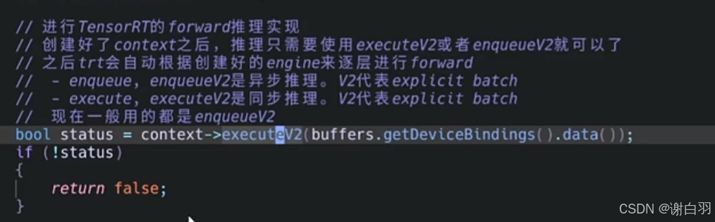
// 进行TensorRT的forward推理实现
// 创建好了context之后,推理只需要使用executeV2或者enqueueV2就可以了
// 之后trt会自动根据创建好的engine来逐层进行forward
// - enqueue, enqueueV2是异步推理。V2代表explicit batch
// - execute, executeV2是同步推理。V2代表explicit batch
// 现在一般用的都是enqueueV2
bool status = context->executeV2(buffers.getDeviceBindings().data());
if (!status)
{
return false;
}
// 将device上forward好的数据copy到host上
buffers.copyOutputToHost();
// postprocess(后处理的实现)
if (!verifyOutput(buffers))
{
return false;
}
return true;
}
/*
* MNIST前处理的实现(这里不详细讲了,主要看一下流程)
* - 读取随机digit数据
* - 分配buffers中的host上的空间
* - 将数据转为浮点数
*/
bool SampleOnnxMNIST::processInput(const samplesCommon::BufferManager& buffers)
{
const int inputH = mInputDims.d[2];
const int inputW = mInputDims.d[3];
// Read a random digit file
srand(unsigned(time(nullptr)));
std::vector<uint8_t> fileData(inputH * inputW);
mNumber = rand() % 10;
readPGMFile(locateFile(std::to_string(mNumber) + ".pgm", mParams.dataDirs), fileData.data(), inputH, inputW);
// Print an ascii representation
sample::gLogInfo << "Input:" << std::endl;
for (int i = 0; i < inputH * inputW; i++)
{
sample::gLogInfo << (" .:-=+*#%@"[fileData[i] / 26]) << (((i + 1) % inputW) ? "" : "\n");
}
sample::gLogInfo << std::endl;
float* hostDataBuffer = static_cast<float*>(buffers.getHostBuffer(mParams.inputTensorNames[0]));
for (int i = 0; i < inputH * inputW; i++)
{
hostDataBuffer[i] = 1.0 - float(fileData[i] / 255.0);
}
return true;
}
/*
* MNIST后处理的实现(同样,这里不详细讲了,主要看一下流程)
* - 分配输出所需要的空间
* - 手动实现一个cpu版本的softmax
* - 输出最大值以及所对应的digit class
*/
bool SampleOnnxMNIST::verifyOutput(const samplesCommon::BufferManager& buffers)
{
const int outputSize = mOutputDims.d[1];
float* output = static_cast<float*>(buffers.getHostBuffer(mParams.outputTensorNames[0]));
float val{0.0f};
int idx{0};
// Calculate Softmax
float sum{0.0f};
for (int i = 0; i < outputSize; i++)
{
output[i] = exp(output[i]);
sum += output[i];
}
sample::gLogInfo << "Output:" << std::endl;
for (int i = 0; i < outputSize; i++)
{
output[i] /= sum;
val = std::max(val, output[i]);
if (val == output[i])
{
idx = i;
}
sample::gLogInfo << " Prob " << i << " " << std::fixed << std::setw(5) << std::setprecision(4) << output[i]
<< " "
<< "Class " << i << ": " << std::string(int(std::floor(output[i] * 10 + 0.5f)), '*')
<< std::endl;
}
sample::gLogInfo << std::endl;
return idx == mNumber && val > 0.9f;
}
samplesCommon::OnnxSampleParams initializeSampleParams(const samplesCommon::Args& args)
{
samplesCommon::OnnxSampleParams params;
if (args.dataDirs.empty()) // Use default directories if user hasn't provided directory paths
{
params.dataDirs.push_back("data/mnist/");
params.dataDirs.push_back("data/samples/mnist/");
}
else // Use the data directory provided by the user
{
params.dataDirs = args.dataDirs;
}
params.onnxFileName = "mnist.onnx";
params.inputTensorNames.push_back("Input3");
params.outputTensorNames.push_back("Plus214_Output_0");
params.dlaCore = args.useDLACore;
params.int8 = args.runInInt8;
params.fp16 = args.runInFp16;
return params;
}
void printHelpInfo()
{
std::cout
<< "Usage: ./sample_onnx_mnist [-h or --help] [-d or --datadir=<path to data directory>] [--useDLACore=<int>]"
<< std::endl;
std::cout << "--help Display help information" << std::endl;
std::cout << "--datadir Specify path to a data directory, overriding the default. This option can be used "
"multiple times to add multiple directories. If no data directories are given, the default is to use "
"(data/samples/mnist/, data/mnist/)"
<< std::endl;
std::cout << "--useDLACore=N Specify a DLA engine for layers that support DLA. Value can range from 0 to n-1, "
"where n is the number of DLA engines on the platform."
<< std::endl;
std::cout << "--int8 Run in Int8 mode." << std::endl;
std::cout << "--fp16 Run in FP16 mode." << std::endl;
}
/*
* 整个main写的比较精简。整体上通过SampleOnnxMNIST这个类把很多底层的实现部分给隐藏了
* 我们在main中所关注的只是
* - "拿到一个onnx"
* - "parse这个onnx来生成trt推理引擎",
* - "推理"
* - "打印输出"
* 所以程序的设计也需要把与这些不相关的不要暴露在外面。提高代码的可读性
* 这个课程后面的代码也基本按照这个思路设计
*/
int main(int argc, char** argv)
{
samplesCommon::Args args;
bool argsOK = samplesCommon::parseArgs(args, argc, argv);
if (!argsOK)
{
sample::gLogError << "Invalid arguments" << std::endl;
printHelpInfo();
return EXIT_FAILURE;
}
if (args.help)
{
printHelpInfo();
return EXIT_SUCCESS;
}
// 创建一个logger用来保存日志。
// 这里需要注意一点,日志一般都是继承nvinfer1::ILogger来实现一个自定义的。
// 由于ILogger有一些函数都是虚函数,所以我们需要自己设计
auto sampleTest = sample::gLogger.defineTest(gSampleName, argc, argv);
sample::gLogger.reportTestStart(sampleTest);
// 创建sample对象,只暴露build和infer接口
SampleOnnxMNIST sample(initializeSampleParams(args));
sample::gLogInfo << "Building and running a GPU inference engine for Onnx MNIST" << std::endl;
// 创建推理引擎
if (!sample.build())
{
return sample::gLogger.reportFail(sampleTest);
}
// 推理
if (!sample.infer())
{
return sample::gLogger.reportFail(sampleTest);
}
return sample::gLogger.reportPass(sampleTest);
}
二、build-model(也叫load model)
1)编译步骤
①构建
make clean
make -j64
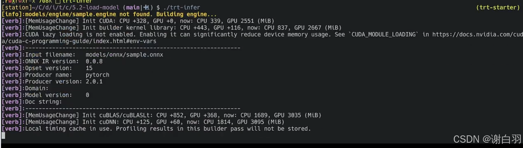
②执行二进制文件,生成模型engine
./trt_infer
2)代码解析
- 整体代码的流程及解析
1)从main函数开始
2)查看logger的实现、model开始调用build函数(老四件套)
3)创建engine然后序列化保存到plan里面,创建runtime(反序列化的东西)
4)把模型导出成类的成员变量
1)从main函数开始,创建model并读取onnx文件,构造函数的时候存储onnx路径
    Model model("models/onnx/sample.onnx");
    if(!model.build()){
        LOGE("ERROR: fail in building model");
        return 0;
    }

//--------------------构造函数
Model::Model(string onnxPath){
    if (!fileExists(onnxPath)) {
        LOGE("%s not found. Program terminated", onnxPath.c_str());
        exit(1);
    }
    mOnnxPath   = onnxPath;
    mEnginePath = getEnginePath(mOnnxPath);
}
2)查看logger的实现,然后老四件套:创建builder、network、config和parser
//自己创建的logger需要继承ILogger,并实现log虚函数
class Logger : public nvinfer1::ILogger{
public:
    virtual void log (Severity severity, const char* msg) noexcept override{
        string str;
        switch (severity){
            case Severity::kINTERNAL_ERROR: str = RED    "[fatal]:" CLEAR;
            case Severity::kERROR:          str = RED    "[error]:" CLEAR;
            case Severity::kWARNING:        str = BLUE   "[warn]:"  CLEAR;
            case Severity::kINFO:           str = YELLOW "[info]:"  CLEAR;
            case Severity::kVERBOSE:        str = PURPLE "[verb]:"  CLEAR;
        }
        if (severity <= Severity::kINFO)
            cout << str << string(msg) << endl;
    }
};


//--------------------------
    auto builder       = make_unique<nvinfer1::IBuilder>(nvinfer1::createInferBuilder(logger));
    auto network       = make_unique<nvinfer1::INetworkDefinition>(builder->createNetworkV2(1));
    auto config        = make_unique<nvinfer1::IBuilderConfig>(builder->createBuilderConfig());
    auto parser        = make_unique<nvonnxparser::IParser>(nvonnxparser::createParser(*network, logger));
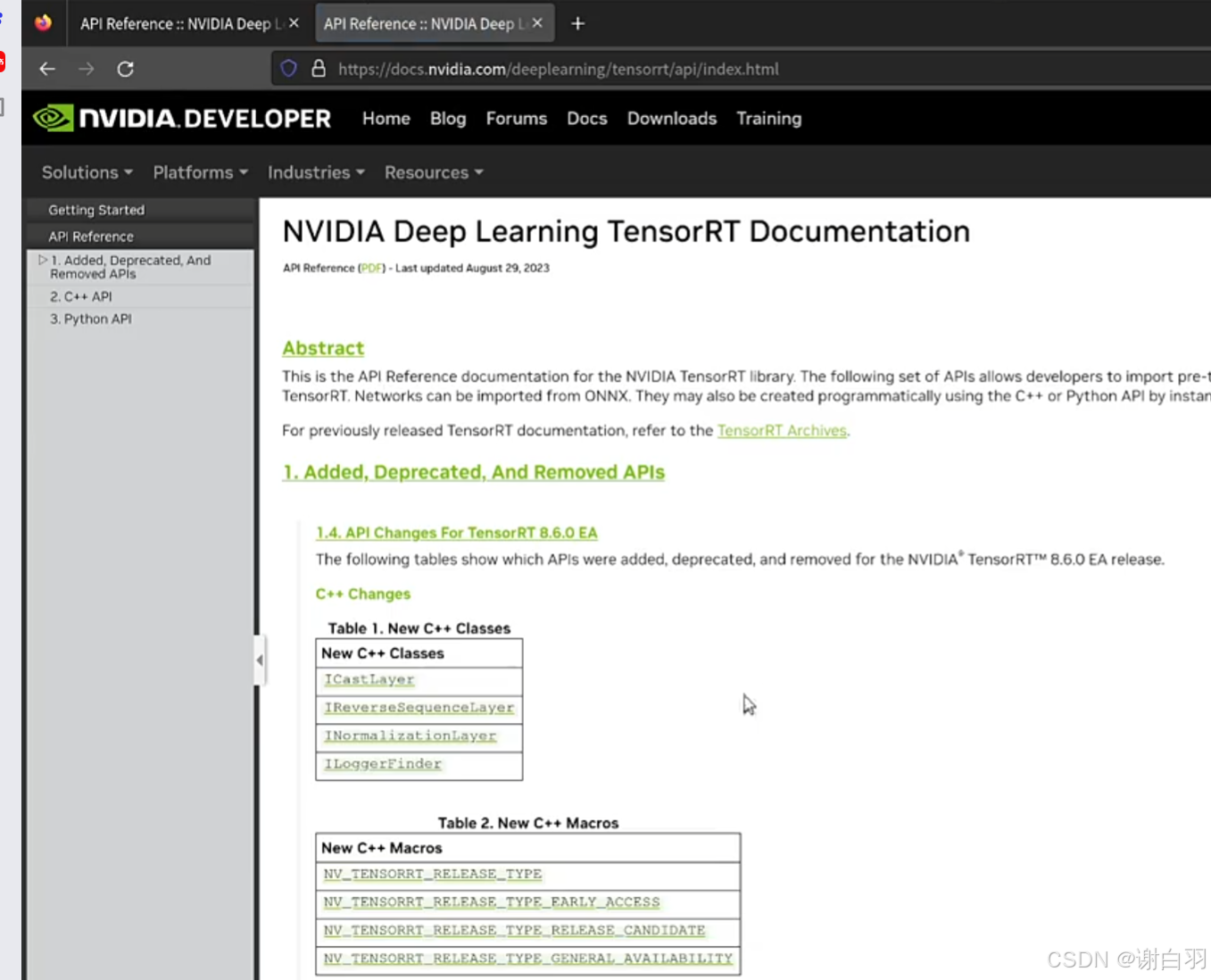
对应的API也可以google搜得到:搜索tensorRT C++ API
3)创建engine然后序列化保存到plan里面,创建runtime(反序列化的东西),打开文件把推理引擎保存下来
备注:序列化成二进制文件,方便保存
    config->setMaxWorkspaceSize(1<<28);

    if (!parser->parseFromFile(mOnnxPath.c_str(), 1)){
        LOGE("ERROR: failed to %s", mOnnxPath.c_str());
        return false;
    }

    auto engine        = make_unique<nvinfer1::ICudaEngine>(builder->buildEngineWithConfig(*network, *config));
    auto plan          = builder->buildSerializedNetwork(*network, *config);//序列化成二进制文件,方便保存
    auto runtime       = make_unique<nvinfer1::IRuntime>(nvinfer1::createInferRuntime(logger));

    auto f = fopen(mEnginePath.c_str(), "wb");
    fwrite(plan->data(), 1, plan->size(), f);
    fclose(f);
4)把模型导出成类的成员变量,并打印输出/输出的维度
    mEngine            = shared_ptr<nvinfer1::ICudaEngine>(runtime->deserializeCudaEngine(plan->data(), plan->size()));
    mInputDims         = network->getInput(0)->getDimensions();
    mOutputDims        = network->getOutput(0)->getDimensions();
    LOG("Input dim is %s", printDims(mInputDims).c_str());
    LOG("Output dim is %s", printDims(mOutputDims).c_str());
- 模型展示(只有一个输入和一个输出)
netron --port 8082 --host 192.168.11.24 sample.onnx

4)代码及布局
-
布局
-
model.hpp
#ifndef __MODEL_HPP__
#define __MODEL_HPP__

// TensorRT related
#include "NvOnnxParser.h"
#include "NvInfer.h"

#include <string>
#include <memory>


class Model{
public:
    Model(std::string onnxPath);
    bool build();
private:
    std::string mOnnxPath;                              //onnx模型路径
    std::string mEnginePath;                            //engine模型路径
    nvinfer1::Dims mInputDims;                          //输入维度
    nvinfer1::Dims mOutputDims;                         //输出维度
    std::shared_ptr<nvinfer1::ICudaEngine> mEngine;     //推理引擎
    bool constructNetwork();
    bool preprocess();
};

#endif // __MODEL_HPP__
- utils.hpp
#ifndef __UTILS_HPP__
#define __UTILS_HPP__

#include <ostream>
#include <string>
#include "NvInfer.h"
#include <stdarg.h>
#include <vector>

#define CUDA_CHECK(call)             __cudaCheck(call, __FILE__, __LINE__)
#define LAST_KERNEL_CHECK(call)      __kernelCheck(__FILE__, __LINE__)

#define LOG(...)                     __log_info(Level::INFO, __VA_ARGS__)
#define LOGV(...)                    __log_info(Level::VERB, __VA_ARGS__)
#define LOGE(...)                    __log_info(Level::ERROR, __VA_ARGS__)

#define DGREEN    "\033[1;36m"
#define BLUE      "\033[1;34m"
#define PURPLE    "\033[1;35m"
#define GREEN     "\033[1;32m"
#define YELLOW    "\033[1;33m"
#define RED       "\033[1;31m"
#define CLEAR     "\033[0m"

enum struct Level {
    ERROR,
    INFO,
    VERB
};

static void __cudaCheck(cudaError_t err, const char* file, const int line) {
    if (err != cudaSuccess) {
        printf("ERROR: %s:%d, ", file, line);
        printf("code:%s, reason:%s\n", cudaGetErrorName(err), cudaGetErrorString(err));
        exit(1);
    }
}

static void __kernelCheck(const char* file, const int line) {
    cudaError_t err = cudaPeekAtLastError();
    if (err != cudaSuccess) {
        printf("ERROR: %s:%d, ", file, line);
        printf("code:%s, reason:%s\n", cudaGetErrorName(err), cudaGetErrorString(err));
        exit(1);
    }
}

static void __log_info(Level level, const char* format, ...) {
    char msg[1000];
    va_list args;
    va_start(args, format);
    int n = 0;

    if (level == Level::INFO) {
        n += snprintf(msg + n, sizeof(msg) - n, YELLOW "[info]: " CLEAR);
    } else if (level == Level::VERB) {
        n += snprintf(msg + n, sizeof(msg) - n, PURPLE "[verb]: " CLEAR);
    } else {
        n += snprintf(msg + n, sizeof(msg) - n, RED    "[error]: " CLEAR);
    }
    n += vsnprintf(msg + n, sizeof(msg) - n, format, args);

    fprintf(stdout, "%s\n", msg);
    va_end(args);

}

bool fileExists(const std::string fileName);
bool fileRead(const std::string &path, std::vector<unsigned char> &data, size_t &size);
std::vector<unsigned char> loadFile(const std::string &path);
std::string printDims(const nvinfer1::Dims dims);
std::string printTensor(float* tensor, int size);
std::string getEnginePath(std::string onnxPath);

#endif //__UTILS_HPP__
三、infer-model(自己写一些反序列化的操作)
1)编译步骤
make  clean
make
./trt-infer
2)代码讲解(主要讲infer做了什么事情,其他部分和上一节差不多)
- 主体流程
1)读取model。然后创建runtime、创建engine、创建context
2)把数据进行host->device传播
3)使用context推理
4)把数据进行device->host传输
步骤拆分
1)读取model。然后创建runtime、创建engine、创建context,并打印维度
- 备注
①IExecutionContext 接口代表了一个执行上下文,它是用于执行推理的核心组件之一。执行上下文包含了网络的所有配置信息,如权重、偏置、激活函数等,以及执行推理所需的所有临时缓冲区。
    /* 1. 读取model => 创建runtime, engine, context */
    if (!fileExists(mEnginePath)) {
        LOGE("ERROR: %s not found", mEnginePath.c_str());
        return false;
    }

    /* 反序列化从文件中读取的数据以unsigned char的vector保存*/
    vector<unsigned char> modelData;
    modelData = loadFile(mEnginePath);

    Logger logger;
    auto runtime     = make_unique<nvinfer1::IRuntime>(nvinfer1::createInferRuntime(logger));
    auto engine      = make_unique<nvinfer1::ICudaEngine>(runtime->deserializeCudaEngine(modelData.data(), modelData.size()));
    auto context     = make_unique<nvinfer1::IExecutionContext>(engine->createExecutionContext());

    auto input_dims   = context->getBindingDimensions(0);
    auto output_dims  = context->getBindingDimensions(1);

    LOG("input dim shape is:  %s", printDims(input_dims).c_str());
    LOG("output dim shape is: %s", printDims(output_dims).c_str());
2)把数据进行host->device传播
    cudaStream_t stream;
    cudaStreamCreate(&stream);

    /* host memory上的数据*/
    float input_host[] = {0.0193, 0.2616, 0.7713, 0.3785, 0.9980, 0.9008, 0.4766, 0.1663, 0.8045, 0.6552};
    float output_host[5];

    /* device memory上的数据*/
    float* input_device = nullptr;
    float* weight_device = nullptr;
    float* output_device = nullptr;

    int input_size = 10;
    int output_size = 5;

    /* 分配空间, 并传送数据从host到device*/
    cudaMalloc(&input_device, sizeof(input_host));
    cudaMalloc(&output_device, sizeof(output_host));
    cudaMemcpyAsync(input_device, input_host, sizeof(input_host), cudaMemcpyKind::cudaMemcpyHostToDevice, stream);
3)模型使用context推理
    float* bindings[] = {input_device, output_device};
    bool success = context->enqueueV2((void**)bindings, stream, nullptr);
4)把数据进行device->host传输
    cudaMemcpyAsync(output_host, output_device, sizeof(output_host), cudaMemcpyKind::cudaMemcpyDeviceToHost, stream);
    cudaStreamSynchronize(stream);

    LOG("input data is:  %s", printTensor(input_host, input_size).c_str());
    LOG("output data is: %s", printTensor(output_host, output_size).c_str());
    LOG("finished inference");
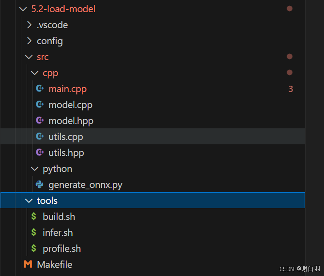
3)整体目录和代码展示
-
目录
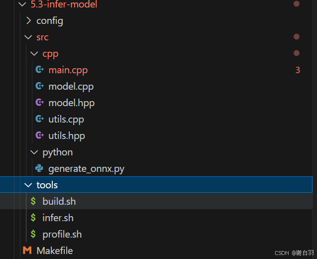
-
main.cpp
#include <iostream>
#include <memory>

#include "model.hpp"
#include "utils.hpp"

using namespace std;

int main(int argc, char const *argv[])
{
    Model model("models/onnx/sample.onnx");
    if(!model.build()){
        LOGE("fail in building model");
        return 0;
    }
    if(!model.infer()){
        LOGE("fail in infering model");
        return 0;
    }
    return 0;
}
四、TensorRT-network-structure(打印模型的架构)
1)编译步骤
make clean
make
./trt-infer
2)不同模型生成前后对比(sample.onnx\resnet50.onnx\vgg16.onnx)
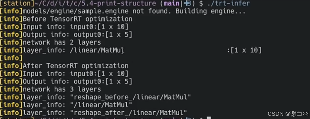
①构建简单的模型:sample.onnx
可以看到
①tensorRT优化之前是2层layer,输入+输出
②tensorRT优化之后是3层layer:reshape_before、linear的Matmul、reshape_after
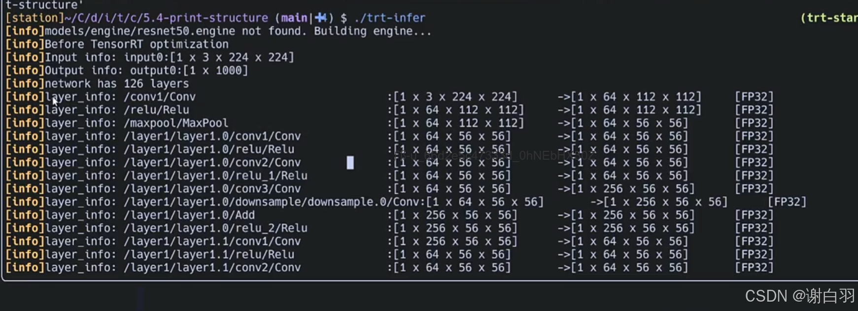
②构建resnet50模型
可以看到优化前网络是126层
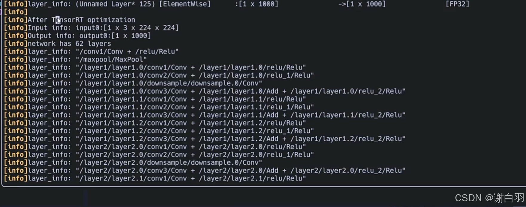
可以看到优化之后是62层
①很多conv+Relu层融合
②很多conv+Add+Relu层融合
等等层融合
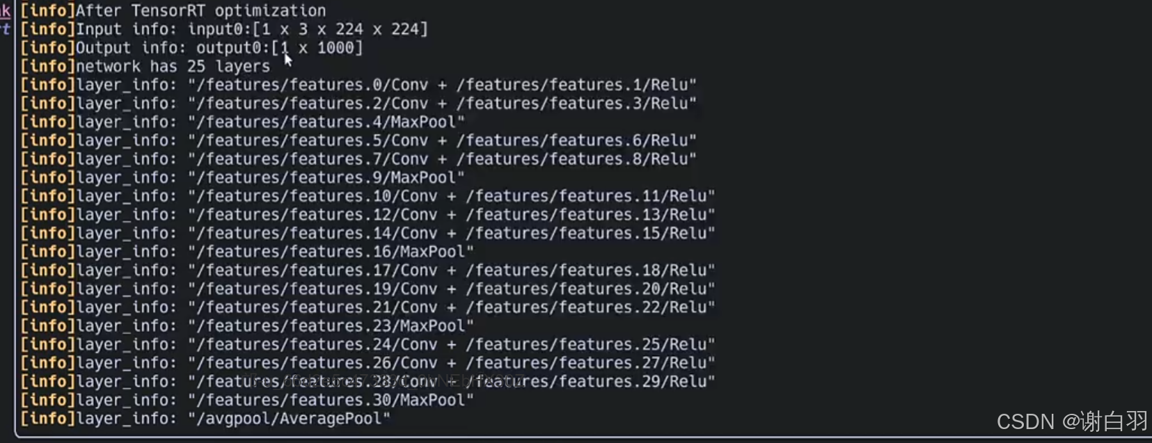
③vgg16模型的创建
可以看到优化前是49层layers
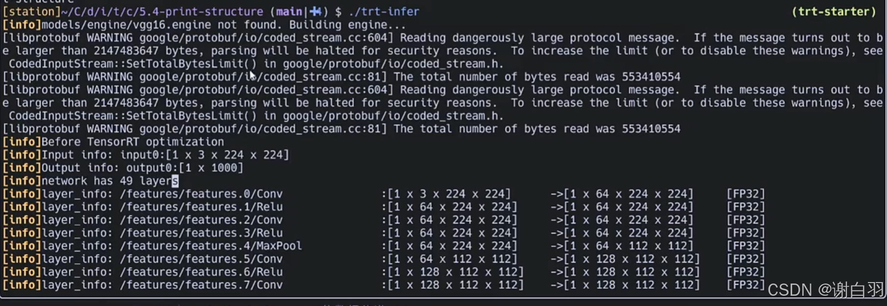
查看优化后的信息,优化后是25层layers
3)相关代码解读
- 重要的类
①如果优化后,那就是打印engine的信息;
②如果优化前,那就是打印network的信息
③打印各个层的信息
- 使用接口
    LOG("Before TensorRT optimization");
    print_network(*network, false);
    LOG("");
    LOG("After TensorRT optimization");
    print_network(*network, true);
    return true;
- 接口代码
void Model::print_network(nvinfer1::INetworkDefinition &network, bool optimized) {
    // ITensor, ILayer, INetwork
    // ICudaEngine, IExecutionContext, IBuilder

    int inputCount = network.getNbInputs();
    int outputCount = network.getNbOutputs();
    string layer_info;

    for (int i = 0; i < inputCount; i++) {
        auto input = network.getInput(i);
        LOG("Input info: %s:%s", input->getName(), printTensorShape(input).c_str());
    }

    for (int i = 0; i < outputCount; i++) {
        auto output = network.getOutput(i);
        LOG("Output info: %s:%s", output->getName(), printTensorShape(output).c_str());
    }

    int layerCount = optimized ? mEngine->getNbLayers() : network.getNbLayers();
    LOG("network has %d layers", layerCount);

    if (!optimized) {
        for (int i = 0; i < layerCount; i++) {
            char layer_info[1000];
            auto layer   = network.getLayer(i);
            auto input   = layer->getInput(0);
            int n = 0;
            if (input == nullptr){
                continue;
            }
            auto output  = layer->getOutput(0);

            LOG("layer_info: %-40s:%-25s->%-25s[%s]",
                layer->getName(),
                printTensorShape(input).c_str(),
                printTensorShape(output).c_str(),
                getPrecision(layer->getPrecision()).c_str());
        }

    } else {
        auto inspector = make_unique<nvinfer1::IEngineInspector>(mEngine->createEngineInspector());
        for (int i = 0; i < layerCount; i++) {
            string info = inspector->getLayerInformation(i, nvinfer1::LayerInformationFormat::kONELINE);

            info = info.substr(0, info.size() - 1);
            LOG("layer_info: %s", info.c_str());
        }
    }
}
4)代码及布局
五、build-model-from-scratch
- 章节目的
①之前的流程都是用tensorRT的parser把onnx解析为tensorRT能识别的数据
②如果我们想看tensorRT导出的模型哪个layer到底是做什么的,需要自己去创建layer,自己创建网络network
③看不同案例(也就是模型)转为engine的时候怎么去做
1)代码流程
- 总体流程
①给模型导入不同的权重
- 具体各个步骤
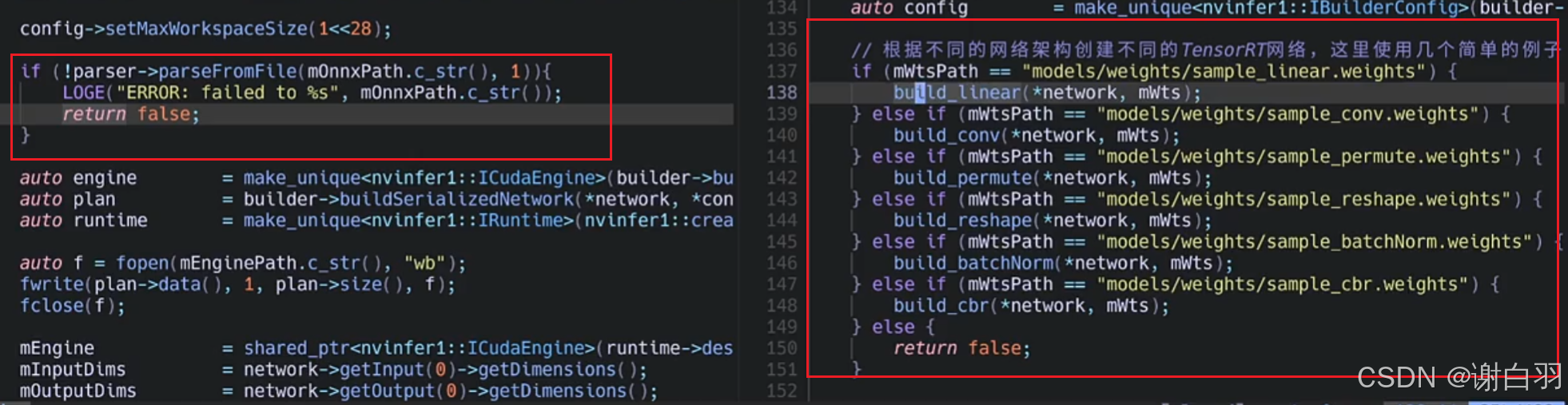
①给模型导入不同的权重
    // Model model("models/weights/sample_linear.weights");
    // Model model("models/weights/sample_conv.weights");
    // Model model("models/weights/sample_permute.weights");
    // Model model("models/weights/sample_reshape.weights");
    // Model model("models/weights/sample_batchNorm.weights");
    // Model model("models/weights/sample_cbr.weights");
    // Model model("models/weights/sample_pooling.weights");
    // Model model("models/weights/sample_upsample.weights");
    // Model model("models/weights/sample_deconv.weights");
    // Model model("models/weights/sample_concat.weights");
    // Model model("models/weights/sample_elementwise.weights");
    // Model model("models/weights/sample_reduce.weights");
    Model model("models/weights/sample_slice.weights");
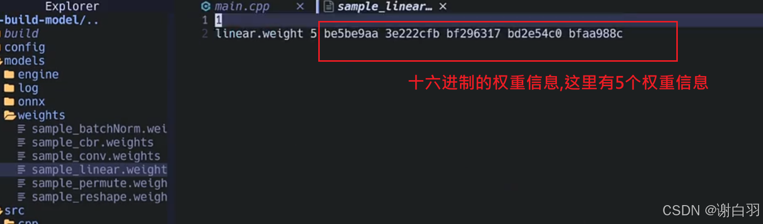
权重信息的展示
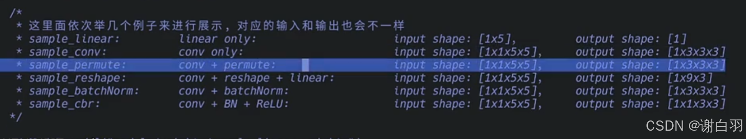
2)不同案例展示及流程讲解
①单纯linear案例
②单纯conv案例
③conv+permute案例
④conv+reshape+linear案例
⑤conv+batchNorm案例
⑥conv+BN+ReLU案例
(1)export_linear.py
-
补充说明
这里可以看到in_feature是5,out_feature是1,表示:
①线性层期望输入的特征向量维度为5,即每次输入的数据有5个特征值,比如在一个简单的房价预测模型中,这5个特征可能是房屋面积、房间数量、房龄、周边配套设施数量、到市中心的距离等。
②经过线性层的变换后,输出的特征向量维度为1,即输出一个数值,在房价预测模型里,这个数值就是预测的房价。 -
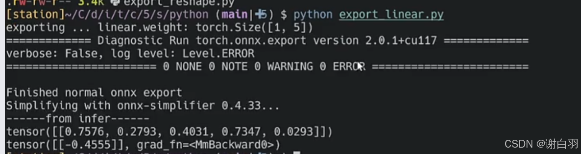
执行代码
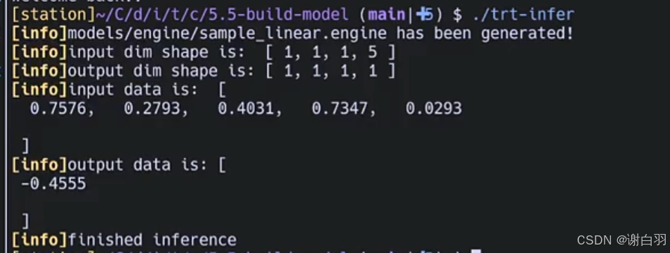
python端测试结果是负的0.4555
C++端输出的结果也是负的0.4555
-
代码讲解
1)之前的build是build_from_onnx(),这里build可以指定从权重构建,也就是build_from_weights
2)先看python是什么形式导出weights
3)再看C++读取weight
4)根据linear函数创建network模型
1)之前的build是build_from_onnx(),这里build可以指定从权重构建,也就是build_from_weights
bool Model::build() {
    if (mOnnxPath != "") {
        return build_from_onnx();
    } else {
        return build_from_weights();
    }
}
2)先看python是什么形式导出weights
# 为了能够让TensorRT读取PyTorch导出的权重,我们可以把权重按照指定的格式导出:
# count  代表多少个权重
# [name][len][weights value in hex mode]  -  [layer的名字][layer权重个数][每个权重的value]
# [name][len][weights value in hex mode]

def export_weight(model):
    current_path = os.path.dirname(__file__)
    f = open(current_path + "/../../models/weights/sample_linear.weights", 'w')
    f.write("{}\n".format(len(model.state_dict().keys())))

    # 我们将权重里的float数据,按照hex16进制的形式进行保存,也就是所谓的编码
    # 可以使用python中的struct.pack
    # 遍历模型的状态字典(state_dict),其中包含了模型的所有参数(权重和偏置)。k 是参数的名称,v 是参数的值(一个张量)
    for k,v in model.state_dict().items():
        print('exporting ... {}: {}'.format(k, v.shape))

        # 将权重转为一维
        # 将参数张量 v 转换为一维数组,并移至 CPU 上,然后转换为 NumPy 数组。
        vr = v.reshape(-1).cpu().numpy()
        f.write("{} {}".format(k, len(vr)))
        # 遍历一维数组中的每个元素,其实也就是打印每个权重信息
        for vv in vr:
            f.write(" ")
            f.write(struct.pack(">f", float(vv)).hex())
        f.write("\n")
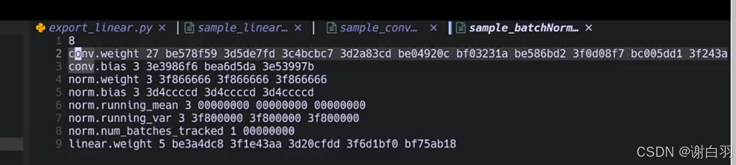
打印的样子
①linear

②conv权重
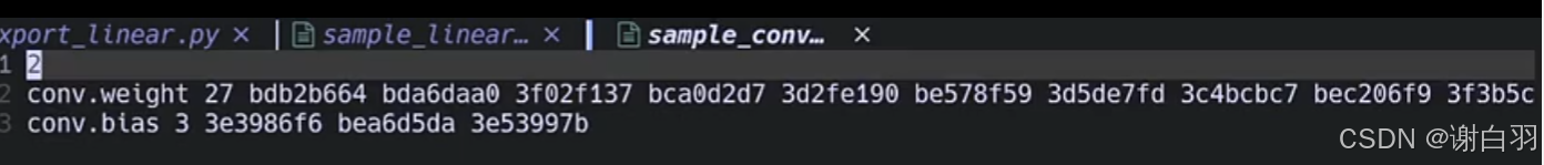
③BatchNormalization
3)再看C++读取weight
①以nvinfer1::Weights的格式导出权重
②对比之前用tensorRT的parser解析的不同点
#加载权重
map<string, nvinfer1::Weights> Model::loadWeights(){
    ifstream f;
    if (!fileExists(mWtsPath)){
        LOGE("ERROR: %s not found", mWtsPath.c_str());
    }

    f.open(mWtsPath);

    int32_t size;
    map<string, nvinfer1::Weights> maps;
    f >> size;

    if (size <= 0) {
        LOGE("ERROR: no weights found in %s", mWtsPath.c_str());
    }

    while (size > 0) {
        nvinfer1::Weights weight;
        string name;
        int weight_length;

        f >> name;
        f >> std::dec >> weight_length;

        uint32_t* values = (uint32_t*)malloc(sizeof(uint32_t) * weight_length);
        for (int i = 0; i < weight_length; i ++) {
            f >> std::hex >> values[i];
        }

        weight.type = nvinfer1::DataType::kFLOAT;
        weight.count = weight_length;
        weight.values = values;

        maps[name] = weight;

        size --;
    }

    return maps;
}
4)根据linear函数创建network模型
- network
/*
 * network
 *
 *  -- input --    ITensor
 *  ---- | ----
 *  ---linear--    Ilayer
 *  ---- | ----
 *  -- output -    ITensor
*/
-
创建network流程
①用network.addInput给网络创建一个输入,返回ITensor
②用network.addFullyConnected设置全连接层,设置linear的一些权重和输入/输出信息
③用fc获取输出并设置名字 -
代码
void Model::build_linear(nvinfer1::INetworkDefinition& network, map<string, nvinfer1::Weights> mWts) {

    auto data          = network.addInput("input0", nvinfer1::DataType::kFLOAT, nvinfer1::Dims4{1, 1, 1, 5});
    auto fc            = network.addFullyConnected(*data, 1, mWts["linear.weight"], {});
    fc->setName("linear1");

    fc->getOutput(0) ->setName("output0");
    network.markOutput(*fc->getOutput(0));
}
- 代码
import torch
import torch.nn as nn
import torch.onnx
import onnxsim
import onnx
import struct
import os

class Model(torch.nn.Module):
    #初始化操作
    def __init__(self):
        super().__init__()
        self.linear = nn.Linear(in_features=5, out_features=1, bias=False)

        #遍历所有模块
        for m in self.modules():
            #1、对于conv卷积层,使用Kaiming正态分布初始化权重,适用于ReLU激活函数,有利于避免梯度消失和梯度爆炸
            if isinstance(m, nn.Conv2d):
                nn.init.kaiming_normal_(m.weight, mode='fan_out', nonlinearity='relu')
            #2、对于全连接层,使用正态分布初始化权重(线性层对输入数据进行线性变换,即通过
            #权重矩阵与输入向量相乘,再加上偏置项得到输出)
            elif isinstance(m, nn.Linear):
                nn.init.normal_(m.weight, mean=0., std=1.)
            #3、对于批量归一化层和组归一化层,使用常量初始化权重改为1和偏置bias改为0
            elif isinstance(m, (nn.BatchNorm2d, nn.GroupNorm)):
                nn.init.constant_(m.wdight, 1)
                nn.init.constant_(m.bias, 0)

    def forward(self, x):
        x = self.linear(x)
        return x


#设置随机数种子是一样的,对于调试和比较不同模型的性能很有帮助
def setup_seed(seed):
    torch.manual_seed(seed)                        #设置CPU上的随机数种子
    torch.cuda.manual_seed_all(seed)               #设置所有GPU上的随机数种子
    torch.backends.cudnn.deterministic = True      #设置cuDNN的随机数种子,保证每次结果一样


# 为了能够让TensorRT读取PyTorch导出的权重,我们可以把权重按照指定的格式导出:
# count
# [name][len][weights value in hex mode]
# [name][len][weights value in hex mode]
# ...

def export_weight(model):
    current_path = os.path.dirname(__file__)
    f = open(current_path + "/../../models/weights/sample_linear.weights", 'w')
    f.write("{}\n".format(len(model.state_dict().keys())))

    # 我们将权重里的float数据,按照hex16进制的形式进行保存,也就是所谓的编码
    # 可以使用python中的struct.pack
    for k,v in model.state_dict().items():
        print('exporting ... {}: {}'.format(k, v.shape))

        # 将权重转为一维
        vr = v.reshape(-1).cpu().numpy()
        f.write("{} {}".format(k, len(vr)))
        for vv in vr:
            f.write(" ")
            f.write(struct.pack(">f", float(vv)).hex())
        f.write("\n")

def export_norm_onnx(input, model):
    current_path = os.path.dirname(__file__)
    file = current_path + "/../../models/onnx/sample_linear.onnx"
    torch.onnx.export(
        model         = model,
        args          = (input,),
        f             = file,
        input_names   = ["input0"],
        output_names  = ["output0"],
        opset_version = 15)
    print("Finished normal onnx export")

    # check the exported onnx model
    model_onnx = onnx.load(file)
    onnx.checker.check_model(model_onnx)

    # use onnx-simplifier to simplify the onnx
    print(f"Simplifying with onnx-simplifier {onnxsim.__version__}...")
    model_onnx, check = onnxsim.simplify(model_onnx)
    assert check, "assert check failed"
    onnx.save(model_onnx, file)

def eval(input, model):
    output = model(input)
    print("------from infer------")
    print(input)
    print(output)

if __name__ == "__main__":
    setup_seed(1)

    input = torch.tensor([[0.7576, 0.2793, 0.4031, 0.7347, 0.0293]])
    model = Model()

    # 以bytes形式导出权重
    export_weight(model);

    # 导出onnx
    export_norm_onnx(input, model);

    # 计算
    eval(input, model)
(2)export_conv.py
-
与前面linear的不同点
①前面反向传播是用的self.linear,这个conv的反向传播是self.conv -
流程
/*
 * network
 *
 *  -- input --    ITensor
 *  ---- | ----
 *  --- conv --    Ilayer
 *  ---- | ----
 *  -- output -    ITensor
*/
- 代码讲解
建立conv
// 最基本的convolution层的创建
void Model::build_conv(nvinfer1::INetworkDefinition& network, map<string, nvinfer1::Weights> mWts) {
    auto data          = network.addInput("input0", nvinfer1::DataType::kFLOAT, nvinfer1::Dims4{1, 1, 5, 5});
    // 3 输出特征图的数量,即卷积核的数量
    // nvinfer1::DimsHW{3, 3}: 卷积核的大小,这里是 3x3
    // mWts["conv.weight"]: 卷积核的权重。
    // mWts["conv.bias"]: 卷积核的偏置
    auto conv          = network.addConvolutionNd(*data, 3, nvinfer1::DimsHW{3, 3}, mWts["conv.weight"], mWts["conv.bias"]);
    conv->setName("conv1");
    // 设置卷积层的步长
    conv->setStride(nvinfer1::DimsHW(1, 1));

    conv->getOutput(0) ->setName("output0");
    // 将卷积层(conv)的输出标记为网络的输出
    network.markOutput(*conv->getOutput(0));
}
- 代码
import torch
import torch.nn as nn
import torch.onnx
import onnxsim
import onnx
import struct
import os

class Model(torch.nn.Module):
    def __init__(self):
        super().__init__()
        #表示输入的参数是1个,输出参数是3个,卷积核是3x3
        self.conv   = nn.Conv2d(1, 3, (3, 3))

        for m in self.modules():
            if isinstance(m, nn.Conv2d):
                nn.init.kaiming_normal_(m.weight, mode='fan_out', nonlinearity='relu')
            elif isinstance(m, nn.Linear):
                nn.init.normal_(m.weight, mean=0., std=1.)
            elif isinstance(m, (nn.BatchNorm2d, nn.GroupNorm)):
                nn.init.constant_(m.wdight, 1)
                nn.init.constant_(m.bias, 0)

    def forward(self, x):
        x = self.conv(x)
        return x

def setup_seed(seed):
    torch.manual_seed(seed)
    torch.cuda.manual_seed_all(seed)
    torch.backends.cudnn.deterministic = True

# 为了能够让TensorRT读取PyTorch导出的权重,我们可以把权重按照指定的格式导出:
# count
# [name][len][weights value in hex mode]
# [name][len][weights value in hex mode]
# ...

def export_weight(model):
    current_path = os.path.dirname(__file__)
    f = open(current_path + "/../../models/weights/sample_conv.weights", 'w')
    f.write("{}\n".format(len(model.state_dict().keys())))

    # 我们将权重里的float数据,按照hex16进制的形式进行保存,也就是所谓的编码
    # 可以使用python中的struct.pack
    for k,v in model.state_dict().items():
        print('exporting ... {}: {}'.format(k, v.shape))

        # 将权重转为一维
        vr = v.reshape(-1).cpu().numpy()
        f.write("{} {}".format(k, len(vr)))
        for vv in vr:
            f.write(" ")
            f.write(struct.pack(">f", float(vv)).hex())
        f.write("\n")

def export_norm_onnx(input, model):
    current_path = os.path.dirname(__file__)
    file = current_path + "/../../models/onnx/sample_conv.onnx"
    torch.onnx.export(
        model         = model,
        args          = (input,),
        f             = file,
        input_names   = ["input0"],
        output_names  = ["output0"],
        opset_version = 15)
    print("Finished normal onnx export")

    # check the exported onnx model
    model_onnx = onnx.load(file)
    onnx.checker.check_model(model_onnx)

    # use onnx-simplifier to simplify the onnx
    print(f"Simplifying with onnx-simplifier {onnxsim.__version__}...")
    model_onnx, check = onnxsim.simplify(model_onnx)
    assert check, "assert check failed"
    onnx.save(model_onnx, file)

def eval(input, model):
    output = model(input)
    print("------from infer------")
    print(input)
    print(output)

if __name__ == "__main__":
    setup_seed(1)

    input = torch.tensor([[[
        [0.7576, 0.2793, 0.4031, 0.7347, 0.0293],
        [0.7999, 0.3971, 0.7544, 0.5695, 0.4388],
        [0.6387, 0.5247, 0.6826, 0.3051, 0.4635],
        [0.4550, 0.5725, 0.4980, 0.9371, 0.6556],
        [0.3138, 0.1980, 0.4162, 0.2843, 0.3398]]]])

    model = Model()

    # 以bytes形式导出权重
    export_weight(model);

    # 导出onnx
    export_norm_onnx(input, model);

    # 计算
    eval(input, model)
(3)export_permute.py
- 流程
/*
 * network
 *
 *  -- input --    ITensor
 *  ---- | ----
 *  --- conv --    ILayer (IConvolutionLayer)
 *  ---- | ----
 *  - permute -    ILayer (IShuffleLayer)
 *  ---- | ----
 *  -- output -    ITensor
*/
- 代码解读
建立conv层和permute层
// shuffle层的创建
void Model::build_permute(nvinfer1::INetworkDefinition& network, map<string, nvinfer1::Weights> mWts) {
    auto data          = network.addInput("input0", nvinfer1::DataType::kFLOAT, nvinfer1::Dims4{1, 1, 5, 5});
    auto conv          = network.addConvolutionNd(*data, 3, nvinfer1::DimsHW{3, 3}, mWts["conv.weight"], mWts["conv.bias"]);
    conv->setName("conv1");
    conv->setStride(nvinfer1::DimsHW(1, 1));

    // 这里的permute层是用来处理维度的,将输入的维度进行重新排列。
    //如果你有一个形状为 (batch_size, channels, height, width) 的四维张量,你可以使用 IShuffleLayer 来将维度重新排列为 (batch_size, height, width, channels)
    auto permute       = network.addShuffle(*conv->getOutput(0));
    //这行代码设置了一个置换,将原来的维度顺序 B, C, H, W 转换为 B, H, W, C。这里的 B 表示批量大小(batch size),C 表示通道数(channels),H 和 W 分别表示高度和宽度。
    permute->setFirstTranspose(nvinfer1::Permutation{0, 2, 3, 1}); // B, C, H, W -> B, H, W, C
    permute->setName("permute1");

    permute->getOutput(0)->setName("output0");
    network.markOutput(*permute->getOutput(0));
}
- 代码
import torch
import torch.nn as nn
import torch.onnx
import onnxsim
import onnx
import struct
import os

class Model(torch.nn.Module):
    def __init__(self):
        super().__init__()
        self.conv   = nn.Conv2d(1, 3, (3, 3))

        for m in self.modules():
            if isinstance(m, nn.Conv2d):
                nn.init.kaiming_normal_(m.weight, mode='fan_out', nonlinearity='relu')
            elif isinstance(m, nn.Linear):
                nn.init.normal_(m.weight, mean=0., std=1.)
            elif isinstance(m, (nn.BatchNorm2d, nn.GroupNorm)):
                nn.init.constant_(m.wdight, 1)
                nn.init.constant_(m.bias, 0)

    def forward(self, x):
        x = self.conv(x)           # B, C, H, W
        x = x.permute(0, 2, 3, 1)  # B, H, W, C
        return x

def setup_seed(seed):
    torch.manual_seed(seed)
    torch.cuda.manual_seed_all(seed)
    torch.backends.cudnn.deterministic = True

# 为了能够让TensorRT读取PyTorch导出的权重,我们可以把权重按照指定的格式导出:
# count
# [name][len][weights value in hex mode]
# [name][len][weights value in hex mode]
# ...

def export_weight(model):
    current_path = os.path.dirname(__file__)
    f = open(current_path + "/../../models/weights/sample_permute.weights", 'w')
    f.write("{}\n".format(len(model.state_dict().keys())))

    # 我们将权重里的float数据,按照hex16进制的形式进行保存,也就是所谓的编码
    # 可以使用python中的struct.pack
    for k,v in model.state_dict().items():
        print('exporting ... {}: {}'.format(k, v.shape))

        # 将权重转为一维
        vr = v.reshape(-1).cpu().numpy()
        f.write("{} {}".format(k, len(vr)))
        for vv in vr:
            f.write(" ")
            f.write(struct.pack(">f", float(vv)).hex())
        f.write("\n")

def export_norm_onnx(input, model):
    current_path = os.path.dirname(__file__)
    file = current_path + "/../../models/onnx/sample_permute.onnx"
    torch.onnx.export(
        model         = model,
        args          = (input,),
        f             = file,
        input_names   = ["input0"],
        output_names  = ["output0"],
        opset_version = 15)
    print("Finished normal onnx export")

    # check the exported onnx model
    model_onnx = onnx.load(file)
    onnx.checker.check_model(model_onnx)

    # use onnx-simplifier to simplify the onnx
    print(f"Simplifying with onnx-simplifier {onnxsim.__version__}...")
    model_onnx, check = onnxsim.simplify(model_onnx)
    assert check, "assert check failed"
    onnx.save(model_onnx, file)

def eval(input, model):
    output = model(input)
    print("------from infer------")
    print(input)
    print(output)

if __name__ == "__main__":
    setup_seed(1)

    input = torch.tensor([[[
        [0.7576, 0.2793, 0.4031, 0.7347, 0.0293],
        [0.7999, 0.3971, 0.7544, 0.5695, 0.4388],
        [0.6387, 0.5247, 0.6826, 0.3051, 0.4635],
        [0.4550, 0.5725, 0.4980, 0.9371, 0.6556],
        [0.3138, 0.1980, 0.4162, 0.2843, 0.3398]]]])

    model = Model()

    # 以bytes形式导出权重
    export_weight(model);

    # 导出onnx
    export_norm_onnx(input, model);

    # 计算
    eval(input, model)
(4)export_reshape.py(导出onnx,view和permute就是一个layer)
- 流程
①原始数据进来就是{1,1,5,5},conv之后就是{1,3,3,3}
②view之后,{B,C,H,W} -> {B,C,L} (H和W结合成L)
③permute,转换C和L位置变成{B,L,C}
/*
 * network
 *
 *  -- input --    ITensor
 *  ---- | ----
 *  --- conv --    ILayer (IConvolutionLayer)
 *  ---- | ----
 *  -- view ---    ILayer (IShuffleLayer)
 *  ---- | ----
 *  - permute -    ILayer (IShuffleLayer)
 *  ---- | ----
 *  -- output -    ITensor
*/
- 具体reshape代码
// shuffle层中处理多次维度上的操作
void Model::build_reshape(nvinfer1::INetworkDefinition& network, map<string, nvinfer1::Weights> mWts) {
    auto data          = network.addInput("input0", nvinfer1::DataType::kFLOAT, nvinfer1::Dims4{1, 1, 5, 5});

    auto conv          = network.addConvolutionNd(*data, 3, nvinfer1::DimsHW{3, 3}, mWts["conv.weight"], mWts["conv.bias"]);
    conv->setName("conv1");
    conv->setStride(nvinfer1::DimsHW(1, 1));

    auto reshape       = network.addShuffle(*conv->getOutput(0));
    // conv之后是B,C,H,W为1,3,3,3;现在第三个参数填-1表示自动补全
    reshape->setReshapeDimensions(nvinfer1::Dims3{1, 3, -1});
    //这里的维度索引是0开始;2, 1表示将原来的第二个维度(索引为1)移动到第三个位置,将原来的第三个维度(索引为2)移动到第二个位置,而第一个维度(索引为0)保持不变
    reshape->setSecondTranspose(nvinfer1::Permutation{0, 2, 1});
    reshape->setName("reshape + permute1");
    // 注意,因为reshape和transpose都是属于iShuffleLayer做的事情,所以需要指明是reshape在前,还是transpose在前
    // 通过这里我们可以看到,在TRT中连续的对tensor的维度的操作其实是可以在TRT中用一个层来处理,属于一种layer fusion优化

    reshape->getOutput(0)->setName("output0");
    network.markOutput(*reshape->getOutput(0));
}
- 代码
import torch
import torch.nn as nn
import torch.onnx
import onnxsim
import onnx
import struct
import os

class Model(torch.nn.Module):
    def __init__(self):
        super().__init__()
        self.conv   = nn.Conv2d(1, 3, (3, 3))

        for m in self.modules():
            if isinstance(m, nn.Conv2d):
                nn.init.kaiming_normal_(m.weight, mode='fan_out', nonlinearity='relu')
            elif isinstance(m, nn.Linear):
                nn.init.normal_(m.weight, mean=0., std=1.)
            elif isinstance(m, (nn.BatchNorm2d, nn.GroupNorm)):
                nn.init.constant_(m.wdight, 1)
                nn.init.constant_(m.bias, 0)

    def forward(self, x):
        x = self.conv(x)                             # B, C, H, W
        x = x.view(x.shape[0], x.shape[1], -1)       # B, C, L
        x = x.permute(0, 2, 1)                       # B, L, C
        return x

def setup_seed(seed):
    torch.manual_seed(seed)
    torch.cuda.manual_seed_all(seed)
    torch.backends.cudnn.deterministic = True

# 为了能够让TensorRT读取PyTorch导出的权重,我们可以把权重按照指定的格式导出:
# count
# [name][len][weights value in hex mode]
# [name][len][weights value in hex mode]
# ...

def export_weight(model):
    current_path = os.path.dirname(__file__)
    f = open(current_path + "/../../models/weights/sample_reshape.weights", 'w')
    f.write("{}\n".format(len(model.state_dict().keys())))

    # 我们将权重里的float数据,按照hex16进制的形式进行保存,也就是所谓的编码
    # 可以使用python中的struct.pack
    for k,v in model.state_dict().items():
        print('exporting ... {}: {}'.format(k, v.shape))

        # 将权重转为一维
        vr = v.reshape(-1).cpu().numpy()
        f.write("{} {}".format(k, len(vr)))
        for vv in vr:
            f.write(" ")
            f.write(struct.pack(">f", float(vv)).hex())
        f.write("\n")

def export_norm_onnx(input, model):
    current_path = os.path.dirname(__file__)
    file = current_path + "/../../models/onnx/sample_reshape.onnx"
    torch.onnx.export(
        model         = model,
        args          = (input,),
        f             = file,
        input_names   = ["input0"],
        output_names  = ["output0"],
        opset_version = 15)
    print("Finished normal onnx export")

    # check the exported onnx model
    model_onnx = onnx.load(file)
    onnx.checker.check_model(model_onnx)

    # use onnx-simplifier to simplify the onnx
    print(f"Simplifying with onnx-simplifier {onnxsim.__version__}...")
    model_onnx, check = onnxsim.simplify(model_onnx)
    assert check, "assert check failed"
    onnx.save(model_onnx, file)

def eval(input, model):
    output = model(input)
    print("------from infer------")
    print(input)
    print(output)

if __name__ == "__main__":
    setup_seed(1)

	# 1,1,5,5
	# 第一个维度的大小为1,表示批量大小(batch size)。在这个例子中,只有一个样本。
    # 第二个维度的大小为1,表示通道数(channels)。在这个例子中,只有一个通道。
    # 第三个维度的大小为5,表示图像的高度。
    # 第四个维度的大小为5,表示图像的宽度。
    input = torch.tensor([[[
        [0.7576, 0.2793, 0.4031, 0.7347, 0.0293],
        [0.7999, 0.3971, 0.7544, 0.5695, 0.4388],
        [0.6387, 0.5247, 0.6826, 0.3051, 0.4635],
        [0.4550, 0.5725, 0.4980, 0.9371, 0.6556],
        [0.3138, 0.1980, 0.4162, 0.2843, 0.3398]]]])

    model = Model()
    model.eval()

    # 以bytes形式导出权重
    export_weight(model);

    # 导出onnx
    export_norm_onnx(input, model);

    # 计算
    eval(input, model)
(5)export_batchNorm.py
- 流程
/*
* network
*
* -- input -- ITensor
* ---- | ----
* --- conv -- ILayer (IConvolutionLayer)
* ---- | ----
* -- BN -- ILayer (IScaleLayer)
* ---- | ----
* -- output - ITensor
*/
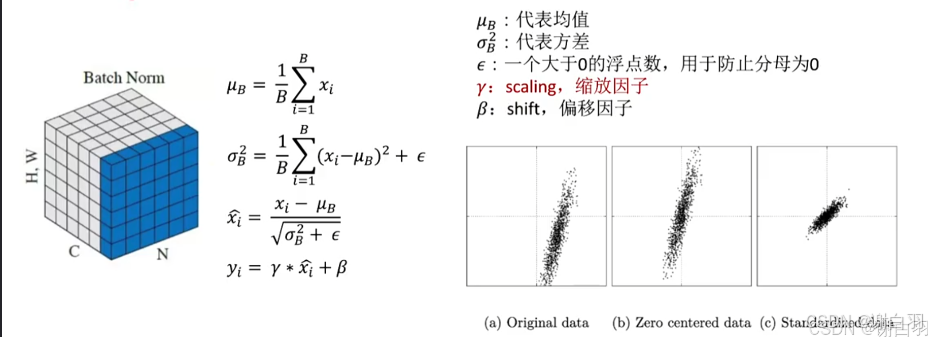
①用IScaleLayer来表示BN
②文档公式
③输入的各个参数
④增加scale,bn是以channel为级别的
①用IScaleLayer来表示BN
②文档公式
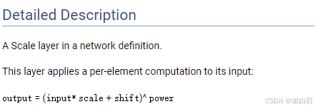
y = (x * scale + shift) ^ pow
③输入的各个参数
    float* gamma   = (float*)mWts["norm.weight"].values;
    float* beta    = (float*)mWts["norm.bias"].values;
    float* mean    = (float*)mWts["norm.running_mean"].values; //平均值
    float* var     = (float*)mWts["norm.running_var"].values;  //方差
    float  eps     = 1e-5;   /默认是10的-5次方,防止分母为0
    nt    count   = mWts["norm.running_var"].count;
④增加scale,bn是以channel为级别的(跟量化差不多,但是量化有nvinfer1::IQuantizeLayer)
    // 创建IScaleLayer并将这些weights传进去,这里使用channel作为scale model
    auto scale = network.addScale(*conv->getOutput(0), nvinfer1::ScaleMode::kCHANNEL, shifts_weights, scales_weights, pows_weights);
    scale->setName("batchNorm1");
- 具体C++实现模型的代码
// 自定义的IScaleLayer来实现BatchNorm的创建
void Model::build_batchNorm(nvinfer1::INetworkDefinition& network, map<string, nvinfer1::Weights> mWts) {
auto data = network.addInput("input0", nvinfer1::DataType::kFLOAT, nvinfer1::Dims4{1, 1, 5, 5});
auto conv = network.addConvolutionNd(*data, 3, nvinfer1::DimsHW{3, 3}, mWts["conv.weight"], mWts["conv.bias"]);
conv->setName("conv1");
conv->setStride(nvinfer1::DimsHW(1, 1));
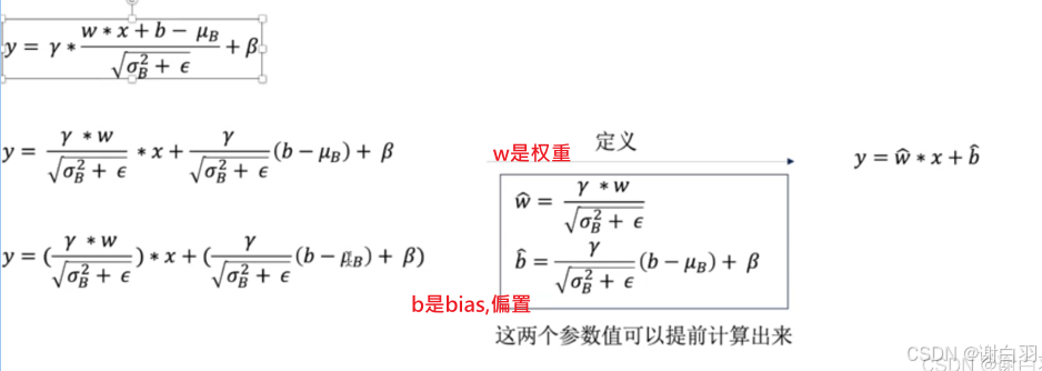
// 因为TensorRT内部没有BatchNorm的实现,但是我们只要知道BatchNorm的计算原理,就可以使用IScaleLayer来创建BN的计算
// IScaleLayer主要是用在quantization和dequantization,作为提前了解,我们试着使用IScaleLayer来搭建于一个BN的parser
// IScaleLayer可以实现: y = (x * scale + shift) ^ pow
float* gamma = (float*)mWts["norm.weight"].values;
float* beta = (float*)mWts["norm.bias"].values;
float* mean = (float*)mWts["norm.running_mean"].values;
float* var = (float*)mWts["norm.running_var"].values;
float eps = 1e-5;
int count = mWts["norm.running_var"].count;
float* scales = (float*)malloc(count * sizeof(float));
float* shifts = (float*)malloc(count * sizeof(float));
float* pows = (float*)malloc(count * sizeof(float));
// 这里具体参考一下batch normalization的计算公式,网上有很多
for (int i = 0; i < count; i ++) {
scales[i] = gamma[i] / sqrt(var[i] + eps);
shifts[i] = beta[i] - (mean[i] * gamma[i] / sqrt(var[i] + eps));
pows[i] = 1.0;
}
// 将计算得到的这些值写入到Weight中
auto scales_weights = nvinfer1::Weights{nvinfer1::DataType::kFLOAT, scales, count};
auto shifts_weights = nvinfer1::Weights{nvinfer1::DataType::kFLOAT, shifts, count};
auto pows_weights = nvinfer1::Weights{nvinfer1::DataType::kFLOAT, pows, count};
// 创建IScaleLayer并将这些weights传进去,这里使用channel作为scale model
auto scale = network.addScale(*conv->getOutput(0), nvinfer1::ScaleMode::kCHANNEL, shifts_weights, scales_weights, pows_weights);
scale->setName("batchNorm1");
scale->getOutput(0) ->setName("output0");
network.markOutput(*scale->getOutput(0));
}
- python代码
可以看到反向传播里面只有conv+bn
    def forward(self, x):
        x = self.conv(x)
        x = self.norm(x)
        return x
- 代码
import torch
import torch.nn as nn
import torch.onnx
import onnxsim
import onnx
import struct
import os

class Model(torch.nn.Module):
    def __init__(self):
        super().__init__()
        self.conv   = nn.Conv2d(1, 3, (3, 3))
        self.act    = nn.ReLU()
        self.norm   = nn.BatchNorm2d(num_features=3)
        self.linear = nn.Linear(in_features=5, out_features=1, bias=False)

        for m in self.modules():
            if isinstance(m, nn.Conv2d):
                nn.init.kaiming_normal_(m.weight, mode='fan_out', nonlinearity='relu')
            elif isinstance(m, nn.Linear):
                nn.init.normal_(m.weight, mean=0., std=1.)
            if isinstance(m, (nn.BatchNorm2d, nn.GroupNorm)):
                nn.init.constant_(m.weight, 1.05)
                nn.init.constant_(m.bias, 0.05)
        # 这里由于weight的初始化是kaiming_normal_,已经达到了标准化了
        # 为了体现BN能够发生改变,将BN的weight和bias都做加0.05处理

    def forward(self, x):
        x = self.conv(x)
        x = self.norm(x)
        return x

def setup_seed(seed):
    torch.manual_seed(seed)
    torch.cuda.manual_seed_all(seed)
    torch.backends.cudnn.deterministic = True

# 为了能够让TensorRT读取PyTorch导出的权重,我们可以把权重按照指定的格式导出:
# count
# [name][len][weights value in hex mode]
# [name][len][weights value in hex mode]
# ...

def export_weight(model):
    current_path = os.path.dirname(__file__)
    f = open(current_path + "/../../models/weights/sample_batchNorm.weights", 'w')
    f.write("{}\n".format(len(model.state_dict().keys())))

    # 我们将权重里的float数据,按照hex16进制的形式进行保存,也就是所谓的编码
    # 可以使用python中的struct.pack
    for k,v in model.state_dict().items():
        print('exporting ... {}: {}'.format(k, v.shape))

        # 将权重转为一维
        vr = v.reshape(-1).cpu().numpy()
        f.write("{} {}".format(k, len(vr)))
        for vv in vr:
            f.write(" ")
            f.write(struct.pack(">f", float(vv)).hex())
        f.write("\n")

def export_norm_onnx(input, model):
    current_path = os.path.dirname(__file__)
    file = current_path + "/../../models/onnx/sample_batchNorm.onnx"
    torch.onnx.export(
        model         = model,
        args          = (input,),
        f             = file,
        input_names   = ["input0"],
        output_names  = ["output0"],
        opset_version = 15)
    print("Finished normal onnx export")

    # check the exported onnx model
    model_onnx = onnx.load(file)
    onnx.checker.check_model(model_onnx)

    # use onnx-simplifier to simplify the onnx
    print(f"Simplifying with onnx-simplifier {onnxsim.__version__}...")
    model_onnx, check = onnxsim.simplify(model_onnx)
    assert check, "assert check failed"
    onnx.save(model_onnx, file)

def eval(input, model):
    output = model(input)
    print("------from infer------")
    print(input)
    print(output)

if __name__ == "__main__":
    setup_seed(1)
    input = torch.tensor([[[
        [0.7576, 0.2793, 0.4031, 0.7347, 0.0293],
        [0.7999, 0.3971, 0.7544, 0.5695, 0.4388],
        [0.6387, 0.5247, 0.6826, 0.3051, 0.4635],
        [0.4550, 0.5725, 0.4980, 0.9371, 0.6556],
        [0.3138, 0.1980, 0.4162, 0.2843, 0.3398]]]])

    model = Model()
    model.eval()
    # 注意,这里有个坑,建议把eval注释掉看看不同
    # 这里需要在export之前进行eval,防止BN层不更新。否则BN层的权重会更新,如果模型中有Dropout也会如此
    # 推荐在以后的导出,以及推理以前都进行eval来固定权重

    # 以bytes形式导出权重
    export_weight(model);


    # 导出onnx
    export_norm_onnx(input, model);

    # 计算
    eval(input, model)
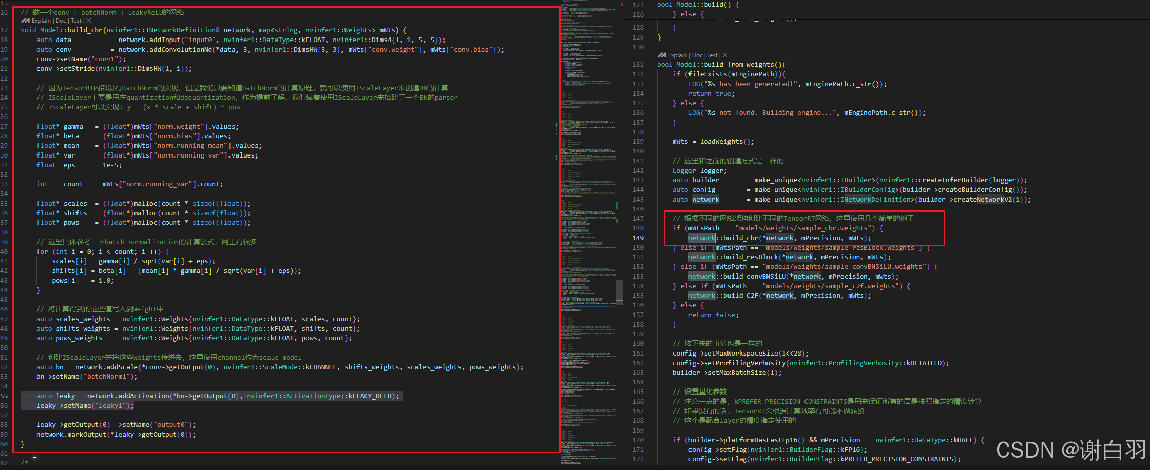
(6)export_cbr.py(conv+bn+relu的结合)
- 流程
/*
 * network
 *
 *  -- input --    ITensor
 *  ---- | ----
 *  --- conv --    ILayer (IConvolutionLayer)
 *  ---- | ----
 *  --  BN   --    ILayer (IScaleLayer)
 *  ---- | ----
 *  -LeakyReLU-    ILayer (IActivationLayer)
 *  ---- | ----
 *  -- output -    ITensor
*/
- 与BN的不同点
①增加了一层layer作为activation
    auto leaky = network.addActivation(*bn->getOutput(0), nvinfer1::ActivationType::kLEAKY_RELU);
    leaky->setName("leaky1");
- 代码
import torch
import torch.nn as nn
import torch.onnx
import onnxsim
import onnx
import struct
import os

class Model(torch.nn.Module):
    def __init__(self):
        super().__init__()
        self.conv   = nn.Conv2d(1, 3, (3, 3))
        self.act    = nn.LeakyReLU()
        self.norm   = nn.BatchNorm2d(num_features=3)
        self.linear = nn.Linear(in_features=5, out_features=1, bias=False)

        for m in self.modules():
            if isinstance(m, nn.Conv2d):
                nn.init.kaiming_normal_(m.weight, mode='fan_out', nonlinearity='relu')
            elif isinstance(m, nn.Linear):
                nn.init.normal_(m.weight, mean=0., std=1.)
            if isinstance(m, (nn.BatchNorm2d, nn.GroupNorm)):
                nn.init.constant_(m.weight, 1.05)
                nn.init.constant_(m.bias, 0.05)
        # 这里由于weight的初始化是kaiming_normal_,已经达到了标准化了
        # 为了体现BN能够发生改变,将BN的weight和bias都做加1处理

    def forward(self, x):
        x = self.conv(x)
        x = self.norm(x)
        x = self.act(x)
        return x

def setup_seed(seed):
    torch.manual_seed(seed)
    torch.cuda.manual_seed_all(seed)
    torch.backends.cudnn.deterministic = True

# 为了能够让TensorRT读取PyTorch导出的权重,我们可以把权重按照指定的格式导出:
# count
# [name][len][weights value in hex mode]
# [name][len][weights value in hex mode]
# ...

def export_weight(model):
    current_path = os.path.dirname(__file__)
    f = open(current_path + "/../../models/weights/sample_cbr.weights", 'w')
    f.write("{}\n".format(len(model.state_dict().keys())))

    # 我们将权重里的float数据,按照hex16进制的形式进行保存,也就是所谓的编码
    # 可以使用python中的struct.pack
    for k,v in model.state_dict().items():
        print('exporting ... {}: {}'.format(k, v.shape))

        # 将权重转为一维
        vr = v.reshape(-1).cpu().numpy()
        f.write("{} {}".format(k, len(vr)))
        for vv in vr:
            f.write(" ")
            f.write(struct.pack(">f", float(vv)).hex())
        f.write("\n")

def export_norm_onnx(input, model):
    current_path = os.path.dirname(__file__)
    file = current_path + "/../../models/onnx/sample_cbr.onnx"
    torch.onnx.export(
        model         = model,
        args          = (input,),
        f             = file,
        input_names   = ["input0"],
        output_names  = ["output0"],
        opset_version = 15)
    print("Finished normal onnx export")

    # check the exported onnx model
    model_onnx = onnx.load(file)
    onnx.checker.check_model(model_onnx)

    # use onnx-simplifier to simplify the onnx
    print(f"Simplifying with onnx-simplifier {onnxsim.__version__}...")
    model_onnx, check = onnxsim.simplify(model_onnx)
    assert check, "assert check failed"
    onnx.save(model_onnx, file)

def eval(input, model):
    output = model(input)
    print("------from infer------")
    print(input)
    print(output)

if __name__ == "__main__":
    setup_seed(1)
    input = torch.tensor([[[
        [0.7576, 0.2793, 0.4031, 0.7347, 0.0293],
        [0.7999, 0.3971, 0.7544, 0.5695, 0.4388],
        [0.6387, 0.5247, 0.6826, 0.3051, 0.4635],
        [0.4550, 0.5725, 0.4980, 0.9371, 0.6556],
        [0.3138, 0.1980, 0.4162, 0.2843, 0.3398]]]])

    model = Model()
    model.eval()
    # 注意,这里有个坑,建议把eval注释掉看看不同
    # 这里需要在export之前进行eval,防止BN层不更新。否则BN层的权重会更新,如果模型中有Dropout也会如此
    # 推荐在以后的导出,以及推理以前都进行eval来固定权重

    # 以bytes形式导出权重
    export_weight(model);


    # 导出onnx
    export_norm_onnx(input, model);

    # 计算
    eval(input, model)
六、build-trt-module(模块化思想)
- 学习目标
①学习tensorRT模块化搭建的思想
②把各种模块搭建成一个模型
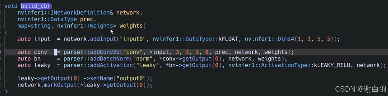
1)cbr(conv+bn+relu)
- 自己实现cbr和NVIDA实现cbr接口的对比
具体实现
2)resblock(resnet网络比较常见)
- 流程
// 做一个residual block:
//       conv0
//       /   \
//      /    conv1
//     |      |
//     |      bn1
//     |      |
//     |     relu1
//     |      |
//     |      |
//     |     conv2
//     |      |
//     |      bn2
//      \    /
//       \  /
//       add2
//        |
//       relu2
//
- 具体构建resblock代码
void build_resBlock(
    nvinfer1::INetworkDefinition& network,
    nvinfer1::DataType prec,
    map<string, nvinfer1::Weights> weights)
{
    auto data  = network.addInput("input0", nvinfer1::DataType::kFLOAT, nvinfer1::Dims4{1, 1, 5, 5});

    auto conv0 = parser::addConv2d("conv0", *data, 3, 3, 1, 1, prec, network, weights);

    auto conv1 = parser::addConv2d("conv1", *conv0->getOutput(0), 3, 3, 1, 1, prec, network, weights);
    auto bn1   = parser::addBatchNorm("norm1", *conv1->getOutput(0), network, weights);
    auto relu1 = parser::addActivation("relu1", *bn1->getOutput(0), nvinfer1::ActivationType::kRELU, network);

    auto conv2 = parser::addConv2d("conv2", *relu1->getOutput(0), 3, 3, 1, 1, prec, network, weights);
    auto bn2   = parser::addBatchNorm("norm2", *conv2->getOutput(0), network, weights);

	//做加法所以操作op是nvinfer1::ElementWiseOperation::kSUM
    auto add2  = parser::addElementWise("add2", *conv0->getOutput(0), *bn2->getOutput(0), nvinfer1::ElementWiseOperation::kSUM, network);
    auto relu2 = parser::addActivation("relu2", *add2->getOutput(0), nvinfer1::ActivationType::kRELU, network);

    relu2->getOutput(0) ->setName("output0");
    network.markOutput(*relu2->getOutput(0));
}
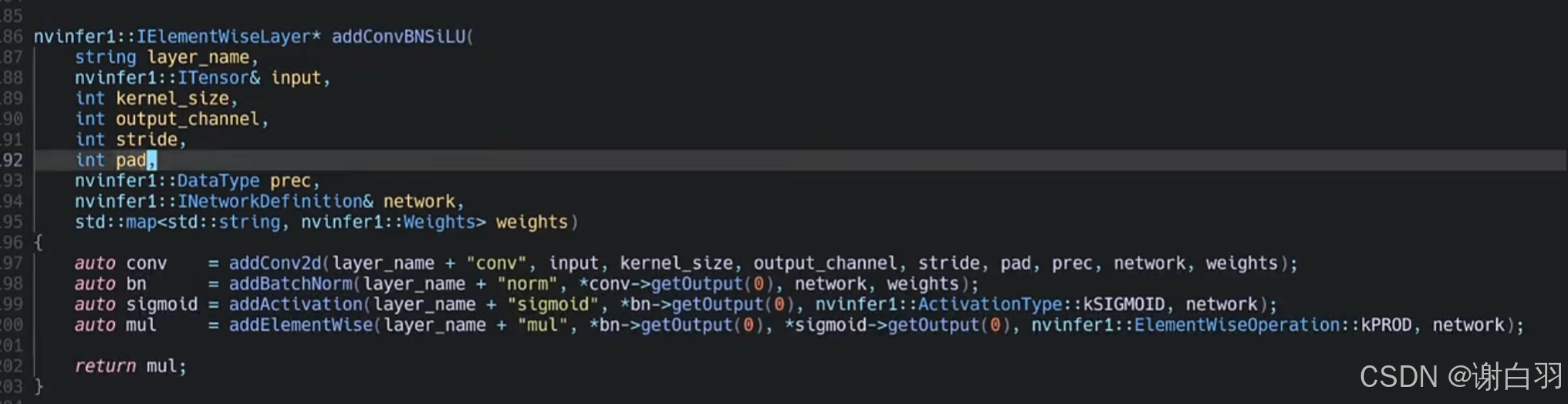
3)convBNSiLU(conv+BN+SeLU)
- 补充关于convBNSiLU的说明
// 做一个conv + bn + SiLU: (yolov8的模块测试)
//        conv
//         |
//         bn
//       /   \
//      |     |
//      |    sigmoid
//      \     /
//       \   /
//        Mul
//
代码(convBNSiLU是包括conv+bn+sigmoid+Mul乘法)
void build_convBNSiLU(
    nvinfer1::INetworkDefinition& network,
    nvinfer1::DataType prec,
    map<string, nvinfer1::Weights> weights)
{
    auto data  = network.addInput("input0", nvinfer1::DataType::kFLOAT, nvinfer1::Dims4{1, 1, 5, 5});

    auto silu  = parser::addConvBNSiLU("", *data, 3, 3, 1, 1, prec, network, weights);


    silu->getOutput(0) ->setName("output0");
    network.markOutput(*silu->getOutput(0));
}
convBNSiLU具体实现
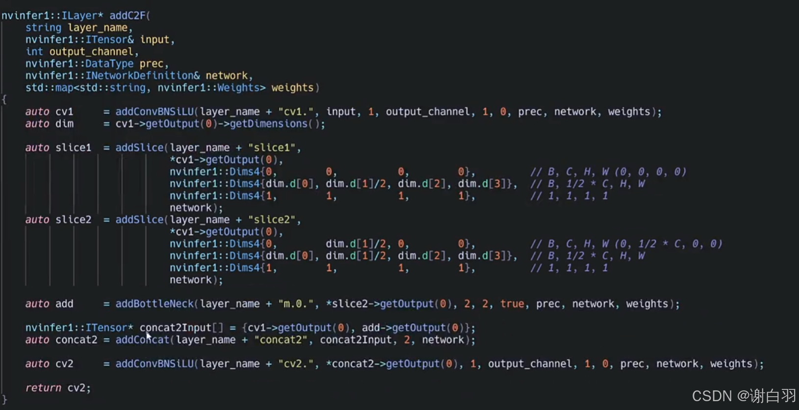
4)c2f
- c2f流程
// 做一个C2F: (yolov8的模块测试)
//        input
//          |
//      convBNSiLU (n * ch)
//       /  |  \
//      /   |   \
//     |    |    |
//     |    | convBNSiLU ( 0.5n * ch)
//     |    |    |
//     |    | convBNSiLU ( 0.5n * ch)
//     |    |    |
//     |    \    /
//     |     \  /
//     |     add (0.5n * ch)
//      \    /
//       \  /
//      Concat (1.5n * ch)
//        |
//    convBNSiLU (n * ch)
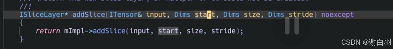
- 接口补充说明
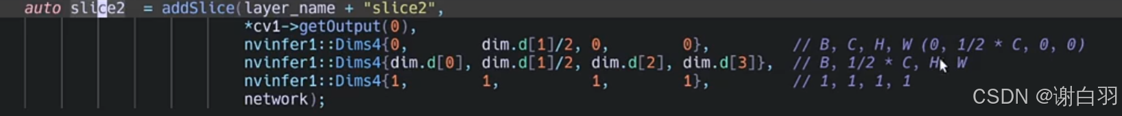
①addSlice
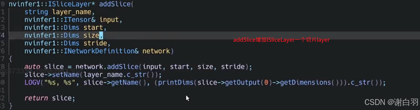
接口作用:把输入的张量按照位移offset和strides步长切分成多个子张量
参数说明:
1)input:输入的张量
2)start:从第几个维度开始切
3)size:输出的维度是多大的
4)stride:切分后模型的步长是多少
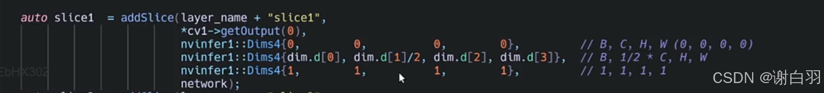
slice1输入参数解释:
1)input是上一步骤conv1的输出,所以是*cv1->getOutput(0)
2)从第零个维度开始切分,所以是{0,0,0,0}
3)切分的size是只对第二个参数,也就是C做channel切分成1/2
4)切分步长和原来不变,步长各个维度仍然是{1,1,1,1}
slice2输入参数解释:
1)input是上一步骤conv1的输出,所以是*cv1->getOutput(0)
2)由于slice1已做切分,所以从slice1改变的地方开始切分,所以是{0,dim.d[1]/2,0,0}
3)切分的size是只对第二个参数,也就是C做channel切分成1/2
4)切分步长和原来不变,步长各个维度仍然是{1,1,1,1}
②addBottleNeck接口
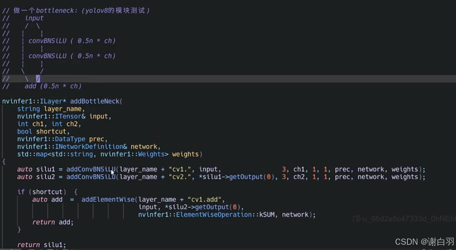
bottleNeck其实就是两个conv的结合,后面流程就是如果是shortcut,那就执行elementWise的加法
③addConcat把conv1的输出、bottleNeck的输出当作两个输入
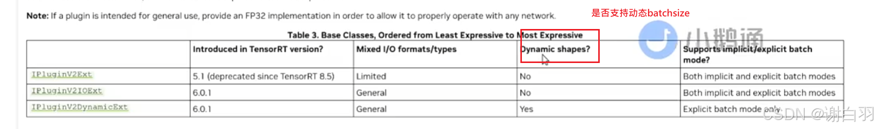
七、custom-trt-module(插件设计)
1)plugin_customScalar
-
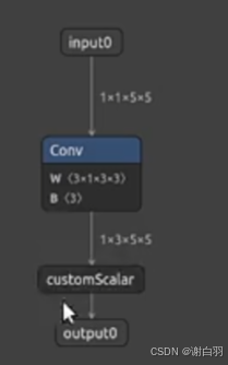
导出onnx查看onnx结构
-
创建插件体现在哪里?
背景:parser在读取解析onnx把数据放到network的时候,我们会读取到onnx里面自定义的算子,如果自定义算子不指定怎么去parse解析的话,tensorRT是无法识别的
解决方法:
自己去写插件plugin
2)plugin_customLeakyReLU
3)自定义插件plugin
-
步骤
1)把插件定义到一个命名空间里面去
2)从onnx里面读取输入的参数后,放到CustomScalarPluginCreator的成员变量mFC里面去,按照键值对读取出来后放到另外一个成员变量mAttrs里面
3)编译过程中会有三次创建插件实例的过程
4)enqueue走前向推理流程,推理函数实现写在cuda代码里面
5)supportsFormatCombination表示tensorRT里面数据的格式,tensorRT的数据格式有很多种,例如CHW\HWC\CHW2\HWC8 -
具体步骤解读
1)把插件定义到一个命名空间里面去
①可以看到这里把CustomScalarPlugin类定义在custom命名空间下面
②可以看到创建了两个类,CustomScalarPluginCreator继承IPluginCreator类,重写创建plugin类和获取版本、获取field名字、创建plugin等初始化操作;CustomScalarPlugin类继承IPluginV2DynamicExt,具体内容是实现scalar这个算子内容的类
2)从onnx里面读取输入的参数后,放到CustomScalarPluginCreator的成员变量mFC里面去,按照键值对读取出来后放到另外一个成员变量mAttrs里面,
CustomScalarPluginCreator::CustomScalarPluginCreator()
{
    /*
     * 每个插件的Creator构造函数需要定制,主要就是获取参数以及传递参数
     * 初始化creator中的PluginField以及PluginFieldCollection
     * - PluginField::            负责获取onnx中的参数
     * - PluginFieldCollection:  负责将onnx中的参数传递给Plugin
    */

    mAttrs.emplace_back(PluginField("scalar", nullptr, PluginFieldType::kFLOAT32, 1));
    mAttrs.emplace_back(PluginField("scale", nullptr, PluginFieldType::kFLOAT32, 1));
    mFC.nbFields = mAttrs.size();
    mFC.fields   = mAttrs.data();
}
3)编译过程中会有三次创建插件实例的过程
    /*
     * 我们在编译的过程中会有大概有三次创建插件实例的过程
     * 1. parse阶段: 第一次读取onnx来parse这个插件。会读取参数信息并转换为TensorRT格式,其实就是调用CustomScalarPlugin构造函数
     * 2. clone阶段: parse完了以后,TensorRT为了去优化这个插件会复制很多副本出来来进行很多优化测试。也可以在推理的时候供不同的context创建插件的时候使用
     * //之前看tensorRT做优化的时候会选择不同blocksize和gridSize来优化插件寻找最好的方案一样的原理
     * 	//调用的构造函数跟第一步一样


     * 3. deseriaze阶段: 将序列化好的Plugin进行反序列化的时候也需要创建插件的实例
    */
4)enqueue走前向推理流程
①element通过对输出维度的累乘知道输入tensor需要的memory空间大小
②调用cuda的函数customScalarImpl
int32_t CustomScalarPlugin::enqueue(
    const PluginTensorDesc* inputDesc, const PluginTensorDesc* outputDesc,
    const void* const* inputs, void* const* outputs,
    void* workspace, cudaStream_t stream) noexcept
{
    /*
     * Plugin的核心的地方。每个插件都有一个自己的定制方案
     * Plugin直接调用kernel的地方
    */
    int nElements = 1;
    for (int i = 0; i < inputDesc[0].dims.nbDims; i++){
        nElements *= inputDesc[0].dims.d[i];
    }

    customScalarImpl(
            static_cast<const float*>(inputs[0]),
            static_cast<float*>(outputs[0]),
            mParams.scalar,
            mParams.scale,
            nElements,
            stream);

    return 0;
}
cuda函数
#include <cuda_runtime.h>
#include <math.h>

__global__ void customScalarKernel(
    const float* input, float* output,
    const float scalar, const float scale, const int nElements)
{
    const int index = blockIdx.x * blockDim.x + threadIdx.x;
    if (index >= nElements)
        return;

    // Perform custom scalar operation(具体核函数内容)
    output[index] = (input[index] + scalar) * scale;
}

void customScalarImpl(const float* inputs, float* outputs, const float scalar, const float scale, const int nElements, cudaStream_t stream)
{
    dim3 blockSize(256, 1, 1);
    dim3 gridSize(ceil(float(nElements) / 256), 1, 1);
    //没有用到共享内存
    customScalarKernel<<<gridSize, blockSize, 0, stream>>>(inputs, outputs, scalar, scale, nElements);
}
5)supportsFormatCombination表示tensorRT里面数据的格式,tensorRT的数据格式有很多种,例如CHW\HWC\CHW2\HWC8( TensorFormat)
bool CustomScalarPlugin::supportsFormatCombination(int32_t pos, const PluginTensorDesc* inOut, int32_t nbInputs, int32_t nbOutputs) noexcept
{
    /*
     * 设置这个Plugin支持的Datatype以及TensorFormat, 每个插件都有自己的定制
     * 作为案例展示,这个customScalar插件只支持FP32,如果需要扩展到FP16以及INT8,需要在这里设置
    */

    switch (pos) {
    case 0:
        return inOut[0].type == DataType::kFLOAT && inOut[0].format == TensorFormat::kLINEAR;
    case 1:
        return inOut[1].type == DataType::kFLOAT && inOut[1].format == TensorFormat::kLINEAR;
    default:
        return false;
    }
    return false;
}
#ifndef __CUSTOM_SCARLAR_PLUGIN_HPP
#define __CUSTOM_SCARLAR_PLUGIN_HPP

#include "NvInferRuntime.h"
#include "NvInferRuntimeCommon.h"
#include <NvInfer.h>
#include <string>
#include <vector>

using namespace nvinfer1;

namespace custom
{
static const char* PLUGIN_NAME {"customScalar"};
static const char* PLUGIN_VERSION {"1"};


/*
* 在这里面需要创建两个类, 一个是普通的Plugin类, 一个是PluginCreator类
*  - Plugin类是插件类,用来写插件的具体实现
*  - PluginCreator类是插件工厂类,用来根据需求创建插件。调用插件是从这里走的
*/

class CustomScalarPlugin : public IPluginV2DynamicExt {
public:
    /*
     * 我们在编译的过程中会有大概有三次创建插件实例的过程
     * 1. parse阶段: 第一次读取onnx来parse这个插件。会读取参数信息并转换为TensorRT格式
     * 2. clone阶段: parse完了以后,TensorRT为了去优化这个插件会复制很多副本出来来进行很多优化测试。也可以在推理的时候供不同的context创建插件的时候使用
     * 3. deseriaze阶段: 将序列化好的Plugin进行反序列化的时候也需要创建插件的实例
    */
    CustomScalarPlugin() = delete; //默认构造函数,一般直接delete
    CustomScalarPlugin(const std::string &name, float scalar, float scale);  //parse, clone时候用的构造函数
    CustomScalarPlugin(const std::string &name, const void* buffer, size_t length); //反序列化的时候用的构造函数

    ~CustomScalarPlugin();

    /* 有关获取plugin信息的方法 */
    const char* getPluginType() const noexcept override;
    const char* getPluginVersion() const noexcept override;
    int32_t     getNbOutputs() const noexcept override;
    size_t      getSerializationSize() const noexcept override;
    const char* getPluginNamespace() const noexcept override;
    DataType    getOutputDataType(int32_t index, DataType const* inputTypes, int32_t nbInputs) const noexcept override;
    DimsExprs   getOutputDimensions(int32_t outputIndex, const DimsExprs* input, int32_t nbInputs, IExprBuilder &exprBuilder) noexcept override;
    size_t      getWorkspaceSize(const PluginTensorDesc *inputs, int32_t nbInputs, const PluginTensorDesc *outputs, int32_t nbOutputs) const noexcept override;

    int32_t     initialize() noexcept override;
    void        terminate() noexcept override;
    void        serialize(void *buffer) const noexcept override;
    void        destroy() noexcept override;
    int32_t     enqueue(const PluginTensorDesc* inputDesc, const PluginTensorDesc* outputDesc, const void* const* ionputs, void* const* outputs, void* workspace, cudaStream_t stream) noexcept override; // 实际插件op执行的地方,具体实现forward的推理的CUDA/C++实现会放在这里面
    IPluginV2DynamicExt* clone() const noexcept override;

    bool        supportsFormatCombination(int32_t pos, const PluginTensorDesc* inOuts, int32_t nbInputs, int32_t nbOutputs) noexcept override; //查看pos位置的索引是否支持指定的DataType以及TensorFormat
    void        configurePlugin(const DynamicPluginTensorDesc* in, int32_t nbInputs, const DynamicPluginTensorDesc* out, int32_t nbOutputs) noexcept override; //配置插件,一般什么都不干
    void        setPluginNamespace(const char* pluginNamespace) noexcept override;

    void        attachToContext(cudnnContext* contextCudnn, cublasContext* contextCublas, IGpuAllocator *gpuAllocator) noexcept override;
    void        detachFromContext() noexcept override;

private:
    const std::string mName;
    std::string       mNamespace;
    struct {
        float scalar;
        float scale;
    } mParams; // 当这个插件op需要有参数的时候,把这些参数定义为成员变量,可以单独拿出来定义,也可以像这样定义成一个结构体
};

class CustomScalarPluginCreator : public IPluginCreator {
public:
    CustomScalarPluginCreator();  //初始化mFC以及mAttrs
    ~CustomScalarPluginCreator();

    const char*                     getPluginName() const noexcept override;
    const char*                     getPluginVersion() const noexcept override;
    const PluginFieldCollection*    getFieldNames() noexcept override;
    const char*                     getPluginNamespace() const noexcept override;
    IPluginV2*                      createPlugin(const char* name, const PluginFieldCollection* fc) noexcept override;  //通过包含参数的mFC来创建Plugin。调用上面的Plugin的构造函数
    IPluginV2*                      deserializePlugin(const char* name, const void* serialData, size_t serialLength) noexcept override;
    void                            setPluginNamespace(const char* pluginNamespace) noexcept override;

private:
    static PluginFieldCollection    mFC;           //接受plugionFields传进来的权重和参数,并将信息传递给Plugin,内部通过createPlugin来创建带参数的plugin
    static std::vector<PluginField> mAttrs;        //用来保存这个插件op所需要的权重和参数, 从onnx中获取, 同样在parse的时候使用
    std::string                     mNamespace;

};

} // namespace custom

#endif __CUSTOM_SCARLAR_PLUGIN_HPP
八、plugin-unit-test(python+cpp,单元测试)
-
总体流程
①通过指定不同维度,不同参数,让uint_test_xxx.python文件做前向推理
②前向推理就是先创建引擎,然后再做inference推理,在做CPU和GPU的结果比较 -
学习目的
①如何再用C++/cuda写完一个plugin后如何快速的做一个单元测试
②如果用python 做API如何创建一个推理引擎,以及做一个前向推理怎么做 -
项目目录
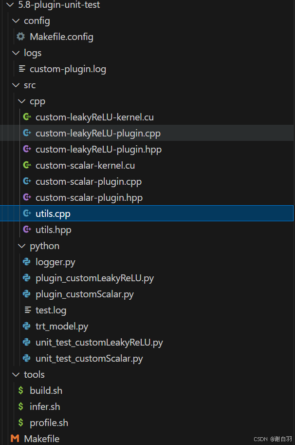
-
各个文件作用
①trt_model.py做推理引擎的创建和前向推理
②logger.py是做一个日志
③unit_test_customLeakyReLU.py是做customLeakyReLU的单元测试 -
单元测试作用
①需要测试去应对很多种情况,比如传入任何scalar和scale都能做正确的计算
②输入的值是tensor,python来测试比较方便
1)编译步骤
①进入到5.8-plugin-unit-test,输入编译指令,在lib目录生成custom-plugin.so
cd 5.8-plugin-unit-test/
bear -- make -j16
②
2)unit_test_customLeakyReLU.py
3)unit_test_customScalar.py
- 代码讲解
①设置日志级别
②uint_test开启不同单元测试
③
④
⑤
①设置日志级别
    test_logger.setLevel(logging.DEBUG)       #日志输出类
    console_handler.setLevel(logging.DEBUG)   #控制台显示的logger是什么样子的
    file_handler.setLevel(logging.INFO)       #在文件显示的日志是什么样子的
②uint_test开启不同单元测试
(1)指定项目目录、so动态库目录、trt引擎目录
(2)ctypes.cdll.LoadLibrary读取动态库
(3)获取tensorRT的接口,接口返回的类型是trt.tensorrt.IPluginV2,从plugin的注册表找一个customScalar
(4)build构建network(C++序列化引擎构建的部分)
engine = build_network(trtFile, shape, plugin)
(5)前向推理
nInput, nIO, bufferH = inference(engine, shape)
(6)校验前向推理结果和CPU结果是否一样
    outputCPU = CustomScalarCPU(bufferH[:nInput], scalar, scale)
    res = validation(nInput, nIO, bufferH, outputCPU)
(7)构建引擎中(build_network)动态shape要指定:最小的动态shape、最优的动态shape、最大的动态shape
        # 为network创建一个dummy的输入,并支持动态shape
        inputT0 = network.add_input("inputT0", trt.float32, [-1 for i in shape])
        profile.set_shape(inputT0.name, [1 for i in shape], [8 for i in shape], [32 for i in shape])
        config.add_optimization_profile(profile)
(8)由于我们只是做单元测试,所以只添加一个插件层plugin
        # 为network添加这个plugin所对应的layer
        pluginLayer = network.add_plugin_v2([inputT0], plugin)
(9)build_network最后步骤是序列化引擎
涉及相关代码
def getCustomScalarPlugin(scalar, scale) -> trt.tensorrt.IPluginV2:
    for c in trt.get_plugin_registry().plugin_creator_list:
        #print(c.name)
        if c.name == "customScalar":
            parameterList = []
            parameterList.append(trt.PluginField("scalar", np.float32(scalar), trt.PluginFieldType.FLOAT32))
            parameterList.append(trt.PluginField("scale", np.float32(scale), trt.PluginFieldType.FLOAT32))
            return c.create_plugin(c.name, trt.PluginFieldCollection(parameterList))
    return None
def unit_test():
    customScalarTest([32], 1, 10)
    customScalarTest([32, 32], 2, 5)
    customScalarTest([16, 16, 16], 1, 3)
    customScalarTest([8, 8, 8, 8], 1, 5)
def customScalarTest(shape, scalar, scale):
    current_path = os.path.dirname(__file__)
    soFile       = current_path + "/../../lib/custom-plugin.so"
    trtFile      = current_path + "/../../models/engine/model-Dim%s.engine" % str(len(shape))
    testCase     = "<shape=%s,scalar=%f,scale=%f>" % (shape, scalar, scale)

    ctypes.cdll.LoadLibrary(soFile)
    plugin = getCustomScalarPlugin(scalar, scale)
    test_logger.info("Test '%s':%s" % (plugin.plugin_type, testCase))

    #################################################################
    ################### 从这里开始是builder的部分 ######################
    #################################################################
    engine = build_network(trtFile, shape, plugin)
    if (engine == None):
        exit()

    #################################################################
    ################### 从这里开始是infer的部分 ########################
    #################################################################
    nInput, nIO, bufferH = inference(engine, shape)

    #################################################################
    ################# 从这里开始是validation的部分 #####################
    #################################################################
    outputCPU = CustomScalarCPU(bufferH[:nInput], scalar, scale)
    res = validation(nInput, nIO, bufferH, outputCPU)

    if (res):
        test_logger.info("Test '%s':%s finish!\n" % (plugin.plugin_type, testCase))
    else:
        test_logger.error("Test '%s':%s failed!\n" % (plugin.plugin_type, testCase))
        exit()
- 具体代码
import ctypes
import os
import numpy as np
import tensorrt as trt
import logging

from trt_model import test_logger, console_handler, file_handler
from trt_model import build_network, inference, validation


def CustomScalarCPU(inputH, scalar, scale):
    return [(inputH[0] + scalar) * scale]

def getCustomScalarPlugin(scalar, scale) -> trt.tensorrt.IPluginV2:
    for c in trt.get_plugin_registry().plugin_creator_list:
        #print(c.name)
        if c.name == "customScalar":
            parameterList = []
            parameterList.append(trt.PluginField("scalar", np.float32(scalar), trt.PluginFieldType.FLOAT32))
            parameterList.append(trt.PluginField("scale", np.float32(scale), trt.PluginFieldType.FLOAT32))
            return c.create_plugin(c.name, trt.PluginFieldCollection(parameterList))
    return None


def customScalarTest(shape, scalar, scale):
    current_path = os.path.dirname(__file__)
    soFile       = current_path + "/../../lib/custom-plugin.so"
    trtFile      = current_path + "/../../models/engine/model-Dim%s.engine" % str(len(shape))
    testCase     = "<shape=%s,scalar=%f,scale=%f>" % (shape, scalar, scale)

    ctypes.cdll.LoadLibrary(soFile)
    plugin = getCustomScalarPlugin(scalar, scale)
    test_logger.info("Test '%s':%s" % (plugin.plugin_type, testCase))

    #################################################################
    ################### 从这里开始是builder的部分 ######################
    #################################################################
    engine = build_network(trtFile, shape, plugin)
    if (engine == None):
        exit()

    #################################################################
    ################### 从这里开始是infer的部分 ########################
    #################################################################
    nInput, nIO, bufferH = inference(engine, shape)

    #################################################################
    ################# 从这里开始是validation的部分 #####################
    #################################################################
    outputCPU = CustomScalarCPU(bufferH[:nInput], scalar, scale)
    res = validation(nInput, nIO, bufferH, outputCPU)

    if (res):
        test_logger.info("Test '%s':%s finish!\n" % (plugin.plugin_type, testCase))
    else:
        test_logger.error("Test '%s':%s failed!\n" % (plugin.plugin_type, testCase))
        exit()

def unit_test():
    customScalarTest([32], 1, 10)
    customScalarTest([32, 32], 2, 5)
    customScalarTest([16, 16, 16], 1, 3)
    customScalarTest([8, 8, 8, 8], 1, 5)

if __name__ == "__main__":
    np.set_printoptions(precision=4, linewidth=200, suppress=True)
    np.random.seed(1)

    test_logger.setLevel(logging.DEBUG)
    console_handler.setLevel(logging.DEBUG)
    file_handler.setLevel(logging.INFO)

    test_logger.info("Starting unit test...")
    unit_test()
    test_logger.info("All tests are passed!!")
九、load-model(从onnx读取一个模型,并把模型序列化,略)
十、文档注释
-
5.4-print-structure:
用tensorRT的API将模型优化前和优化后的模型架构打印出来 -
5.5-build-model
如何从pytorch导出onnx到,导出tensorRT的流程 -
5.6-build-sub-graph
如何用tensorRT的API去搭建一些小模块去拼凑大的网络 -
5.7-custom-trt-plugin
如何创建plugin该怎么做 -
5.8-plugin-unit-test
用python api去搭建tensorRT模型,把C++写的插件导入进来去做单元测试


 328
328

 被折叠的 条评论
为什么被折叠?
被折叠的 条评论
为什么被折叠?
 到【灌水乐园】发言


