


- 代码和论文下载:在paperwithcode网站搜索HRNet

代码下载到自己的电脑:

代码:根据自己笔记本电脑的情况重新改写了源代码(不完整,主要是为了分析生成器结构写的),去掉了一些无关紧要的内容,但是主体是没变的。所以后面的讲解时根据改写的代码分析。
链接:https://pan.baidu.com/s/13LiJZWraoxLW7l6cdFEjpQ
提取码:hrug
train.py
当前的工作目录是HRNet_project,执行train.py训练模型的函数后会进入main.py

main.py关键部分详解
读取配置文件.yaml中的变量,这些变量是模型搭建中需要的
    # the setting of config
    args = parse_args()
    config = Config(args)
    config.project_path = os.path.dirname(__file__)
    config.mode = mode
关于配置文件路径输入是在命令行方式parse_args()中输入的.由于我是在win上调试并分析,所以我把导入方式设置为默认并固定了:
def parse_args():
    parser = argparse.ArgumentParser(description='Train segmentation network')
    parser.add_argument('--yaml_path',
                        help='experiment configure file name',
                        # required=True,
                        default=os.path.dirname(__file__)+'\experiments\cityscapes\seg_hrnet_w48_train_512x1024_sgd_lr1e-2_wd5e-4_bs_12_epoch484.yaml',
                        type=str)
    args = parser.parse_args()
    return args
通过ctrl+B进入config = Config(args)中的Config()函数,它是为了读取.yaml文件内容的:
class Config(dict):
    def __init__(self, args):
        # open the file of .yaml
        with open(args.yaml_path, 'r') as f:
            self._dict = yaml.load(f.read()) # Load the dictionary
            self.args = vars(args)  # change to the type of dict

    # __getattr__:当使用点号获取实例属性时,如果属性不存在就自动调用__getattr__方法
    def __getattr__(self, name):
        if self._dict.get(name) is not None:
            return self._dict[name]

        if self.args.get(name) is not None:
            return self.args[name]
        return None

运算环境的选择GPU/CPU,如果有NVIDIA的GPU,就可以用并行运算的cuda库去管理它,而cudnn是加速cuda并行运算能力的,可以自行选择。(由于我笔记本配置太低,我先注释了)
    # device setting: if the GPU is None
    if torch.cuda.is_available():
        os.environ['CUDA_VISIBLE_DEVICES'] = ','.join(str(e) for e in config.GPUs)
        config.DEVICE = torch.device("cuda")
        # # cudnn related setting
        # cudnn.benchmark = True
        # cudnn.deterministic = False
        # cudnn.enabled = True
    else:
        config.DEVICE = torch.device("cpu")
    print('DEVICE is:', config.DEVICE)
初始化HRNet模型
    # build and initialize the model
    model = HRNet(config)
训练集的准备:
链接:https://pan.baidu.com/s/1dxsVOOZ1RC7c-obM23fHIg
提取码:kmrl
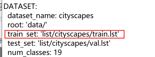
将数据下载好后,再将其中的gtFine和leftImg8bit文件夹放入到源代码中的data目录下,具体data中的目录结构如下所示:
E:.
├── cityscapes
│   ├── gtFine
│   │   ├── test
│   │   ├── train
│   │   └── val
│   └── leftImg8bit
│       ├── test
│       ├── train
│       └── val
├── list
│   ├── cityscapes
│   │   ├── test.lst
│   │   ├── trainval.lst
│   │   └── val.lst
│   ├── lip
│   │   ├── testvalList.txt
│   │   ├── trainList.txt
│   │   └── valList.txt
自定义数据接口和设定数据导入方式:
# prepare dataset
if config.mode == 1:
    config.train_dataset = dataset.Cityscapes(
        root= os.path.join(config.project_path, config.DATASET["root"]),
        list_path=config.DATASET["train_set"],
        num_samples = None,    # 要提取样本数
        num_classes = config.DATASET["num_classes"],
        multi_scale= True,
        flip= True,
        ignore_label= 255,
        base_size= config.TRAIN["base_size"],
        crop_size= config.TRAIN["crop_size"],
        downsample_rate= 1,
        scale_factor= 16)

    config.trainloader = torch.utils.data.DataLoader(
        config.train_dataset,
        batch_size = config.TRAIN["batch_size_per_gpu"] * len(config.GPUs),
        shuffle=True,
        # shuffle = False,
        num_workers = config.WORKERS)
“class Cityscapes(BaseDataset):” 中数据读取的过程:
在配置文件中的DATASET变量有设定训练集的的路径train.lst, 该文件的存储格式是一行为一个样本,每个样本的格式是图像路劲与对应标签路径的组合:[image_path label_path]
将train.lst中的内容一行一行的读出来,并以空格进行切分:
        # .txt/.lst数据获取:打开文件,以空格分割每一行(注意:不要有空行)
        self.img_list = [line.strip().split() for line in open(root + list_path)]

由于img_list中只记录了image和label的路径,如果我们还想加入某些变量,如这一对样本的name等:
        # 添加信息:sample{image_path,label_path, lable_name}
        self.files = self.read_files()
files[i] = {“img”: image_path_i,“label”: label_path_i,“name”: name_i }
            for item in self.img_list:
                image_path, label_path = item
                name = os.path.splitext(os.path.basename(label_path))[0]
                files.append({
                    "img": image_path,
                    "label": label_path,
                    "name": name,
                })
这是获取.lst中的全部训练样本,一般情况是这样的。如果全部样本数是10000对,但是我只想把之中的前200对样本用于训练,则可以通过变量num_samples实现:
# files=[{sample1},{sample2},{sample3},...] , num_samples:提取的样本数
if num_samples:
     self.files = self.files[:num_samples]
下面就是对**def getitem(self, index):**的分析:
 def __getitem__(self, index):
        item = self.files[index]
        name = item["name"]
        image = cv2.imread(os.path.join(self.root, 'cityscapes', item["img"]),
                           cv2.IMREAD_COLOR)
        size = image.shape

        if 'test' in self.list_path:
            image = self.input_transform(image)
            image = image.transpose((2, 0, 1))

            return image.copy()

        label = cv2.imread(os.path.join(self.root, 'cityscapes', item["label"]),
                           cv2.IMREAD_GRAYSCALE)
        label = self.convert_label(label)

        image, label = self.gen_sample(image, label,
                                       self.multi_scale, self.flip)

        return image.copy(), label.copy(), np.array(size), name
image:
# 以BGR格式读取图像
image = cv2.imread(os.path.join(self.root, 'cityscapes', item["img"]),
                       cv2.IMREAD_COLOR)
size: [ H , W ] = 1024*2048

只是读取的原图,需要进行处理后用于训练:
def gen_sample(self, image, label,
              multi_scale=True, is_flip=True):
   if multi_scale:
       rand_scale = 0.5 + random.randint(0, self.scale_factor) / 10.0
       image, label = self.multi_scale_aug(image, label,
                                           rand_scale=rand_scale)

   image = self.input_transform(image)
   label = self.label_transform(label)

   image = image.transpose((2, 0, 1))

   if is_flip:
       flip = np.random.choice(2) * 2 - 1
       image = image[:, :, ::flip]
       label = label[:, ::flip]

   if self.downsample_rate != 1:
       label = cv2.resize(label,
                          None,
                          fx=self.downsample_rate,
                          fy=self.downsample_rate,
                          interpolation=cv2.INTER_NEAREST)
   return image, label
先将原图进行等比例[ 0.5, 2.0]的放缩 “multi_scale=True”。 由于原图很大(1024*2048),缩小后的图像较原图会更清晰,也更细腻。由于裁剪之前是随机的放缩,自然也可能会出现放大的情况。这种随机性可以增加模型的泛化(适应)能力。
# 先放缩,后裁剪
if multi_scale:
   rand_scale = 0.5 + random.randint(0, self.scale_factor) / 10.0
   image, label = self.multi_scale_aug(image, label,
                                       rand_scale=rand_scale)

训练样本的大小设定为 crop_size: [512, 1024],故需要对上面放缩后的图片进行裁剪。为什么不直接对原图进行裁剪的原因就是想增加模型对不同分辨率数据的适应能力(即泛化能力)。

读取的图片类型image.dtype=“uint8”,训练的数据格式通常为32位。而归一化/标准化后可以提升模型的收敛速度:
image = self.input_transform(image)
def input_transform(self, image):
       # 数据格式转换
       image = image.astype(np.float32)[:, :, ::-1]
       # 归一化:把数变为(0,1)之间的小数
       image = image / 255.0
       # 标准化:将数据按比例缩放,使之落入一个小的特定区间
       image -= self.mean
       image /= self.std
       # cv2读出的图片存储使用的是:H×W×C,需要转换成C×H×W
       image = image.transpose((2, 0, 1))
       return image
图像传统的增强方法之对图像进行翻转:
 if is_flip:
     # -1: 将图像向右翻转180°; 1: 原图
     flip = np.random.choice(2) * 2 - 1  # -1/1
     image = image[:, :, ::flip]
     label = label[:, ::flip]
每导入一个items={image, label, size, name},就会包含这4项。WORKERS为什么是0参考:https://blog.csdn.net/u013066730/article/details/97808471
config.testloader = dataset.Cityscapes(
    config.test_dataset,
    batch_size = config.TEST["batch_size_per_gpu"]*len(config.GPUs),
    shuffle= False,
    num_workers= config.WORKERS)
label:
# 以灰度图像格式读取图像
label = cv2.imread(os.path.join(self.root, 'cityscapes', item["label"]),
                   cv2.IMREAD_GRAYSCALE)
size: [ H , W ] = 1024*2048

处理操作:
def convert_label(self, label, inverse=False):
       temp = label.copy()
       #
       if inverse:
           for v, k in self.label_mapping.items():
               label[temp == k] = v
       else:
           for k, v in self.label_mapping.items():  # (k ,v) = (-1 , ignore_label=255)
               label[temp == k] = v
       return label
self.label_mapping = {-1: ignore_label, 0: ignore_label,
                        1: ignore_label, 2: ignore_label,
                        3: ignore_label, 4: ignore_label,
                        5: ignore_label, 6: ignore_label,
                        7: 0, 8: 1, 9: ignore_label,
                        10: ignore_label, 11: 2, 12: 3,
                        13: 4, 14: ignore_label, 15: ignore_label,
                        16: ignore_label, 17: 5, 18: ignore_label,
                        19: 6, 20: 7, 21: 8, 22: 9, 23: 10, 24: 11,
                        25: 12, 26: 13, 27: 14, 28: 15,
                        29: ignore_label, 30: ignore_label,
                        31: 16, 32: 17, 33: 18}
ArcGis中查看label的灰度图像,发现它们的像素值区间都在[0,33]间,如下图所示:

"inverse=False"是否将像素区间倒置,下图就是倒置后的结果:

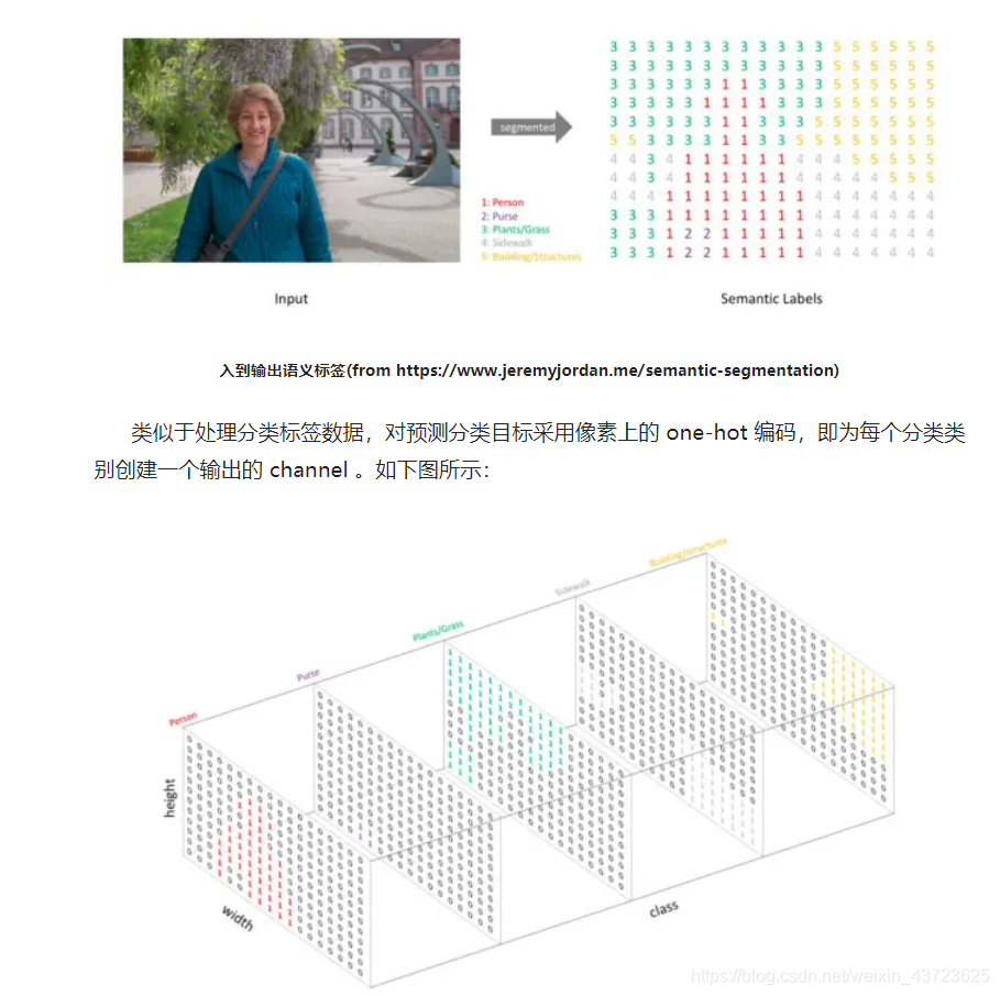
图像的多分类问题中,如果以像素值作为分类的标志,那么就会有34类。而我们不需要则会么多的分类标签,就需要合并一些标签。这就用到了self.label_mapping变量进行像素值的修改(最终的类别数num_classes: 19):


关于label的 "image, label = self.gen_sample(image, lab , self.multi_scale, self.flip)"操作,就不介绍了,因为image中有说明。
# select model
if config.mode == 1:
   self.Train_Model = Train_Model(config).to(config.DEVICE)

class Train_Model(BaseModel):
   def __init__(self, config):
       super(Train_Model, self).__init__(config)

       # initialize the network
       self.generator = Generator(config)
生成器介绍:Generator
由于笔记本配置有限,最多扩展到stage3。其实stage4的操作都是类似的。

其中关于layer1是由四个残差单元构成,其的结构如下:

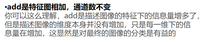
最后输出的通道数为num_class=19,这是在为每个分类创建一个输出的channel。参考下图理解:
生成器部分,已经理解得差不多了。由于自己是研究图像合成的,后面的部分就先不想看了。可以参考另一篇博客:https://blog.csdn.net/u013066730/article/details/97787207


 2252
2252


 被折叠的 条评论
为什么被折叠?
被折叠的 条评论
为什么被折叠?
 到【灌水乐园】发言


