数据挖掘——seaborn

import seaborn as sns
import numpy as np
import pandas as pd
import matplotlib.pyplot as plt

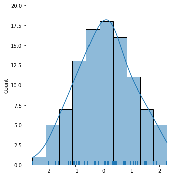
绘制单变量分布

# seaborn.distplot(a, bins=None, hist=True, kde=True, rug=False, fit=None, color=None)
# 上述函数中常用参数的含义如下：
# (1) a：表示要观察的数据，可以是 Series、一维数组或列表。
# (2) bins：用于控制条形的数量。
# (3) hist：接收布尔类型，表示是否绘制(标注)直方图。
# (4) kde：接收布尔类型，表示是否绘制高斯核密度估计曲线。
# (5) rug：接收布尔类型，表示是否在支持的轴方向上绘制rugplot。

np.random.seed(0)#确定随机数生成器中生成的数据是一致的
arr = np.random.randn(100)
sns.displot(arr,bins=10,kde=True,rug=True)

<seaborn.axisgrid.FacetGrid at 0x1dcb31164f0>

​

​

绘制双变量分布

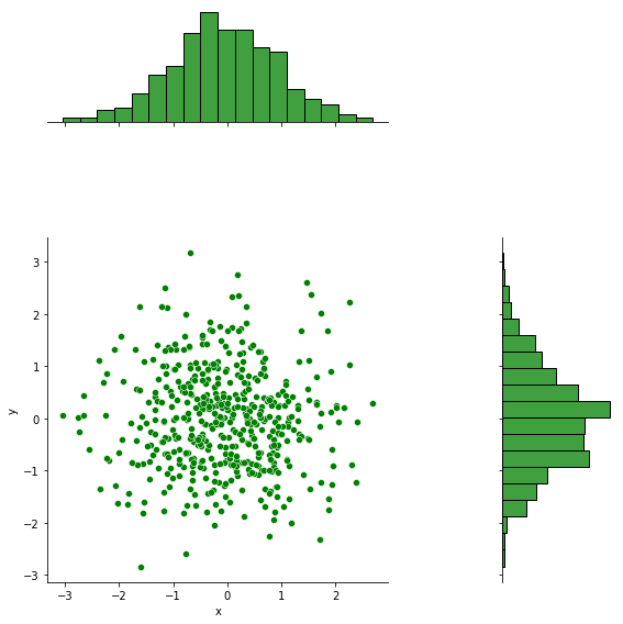
绘制散点图

# 创建DataFrame数据
df = pd.DataFrame({"x":np.random.randn(500),"y":np.random.randn(500)})

df.head()

	x	y
0	1.883151	-1.550429
1	-1.347759	0.417319
2	-1.270485	-0.944368
3	0.969397	0.238103
4	-1.173123	-1.405963

# jointplot()函数的语法格式如下。
# seaborn.jointplot(x, y, data=None,
# kind='scatter', stat_func=None, color=None,
# ratio=5, space=0.2, dropna=True)
# 上述函数中常用参数的含义如下：
# (1) kind：表示绘制图形的类型。
# (2) stat_func：用于计算有关关系的统计量并标注图。
# (3) color：表示绘图元素的颜色。
# (4) size：用于设置图的大小(正方形)。
# (5) ratio：表示中心图与侧边图的比例。该参数的值越大，则中心图的占比会越大。
# (6) space：用于设置中心图与侧边图的间隔大小。
# 下面以散点图、二维直方图、核密度估计曲线为例，为大家介绍如何使用 Seaborn绘制这些图形。

sns.jointplot(x="x",y="y",data=df,kind="scatter",color="green",height=8,ratio=2,space=1)

<seaborn.axisgrid.JointGrid at 0x1dcb885e910>

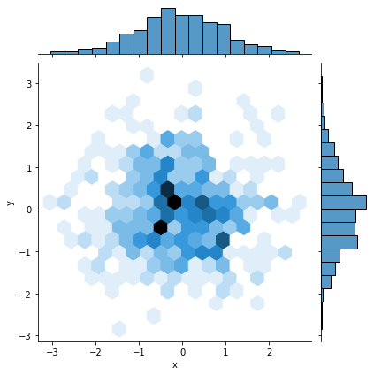
绘制二维直方图

# 颜色越深代表数据越密集  颜色越浅代表数据越稀疏
sns.jointplot(x="x",y="y",data=df,kind="hex")

<seaborn.axisgrid.JointGrid at 0x1dcb8938160>

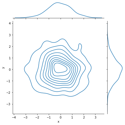
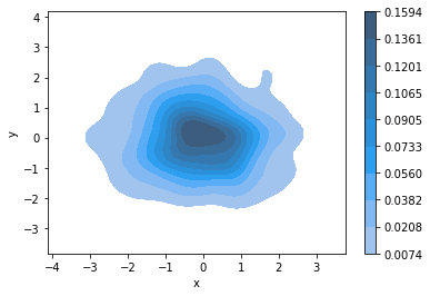
绘制核密度估计度

# 看等高线的颜色深浅来绘制  颜色越深代表数据越密集  颜色越浅代表数据越稀疏
sns.jointplot(x="x",y="y",data=df,kind="kde")

<seaborn.axisgrid.JointGrid at 0x1dcb6f31130>

sns.kdeplot(x="x",y="y",data=df,shade=True,cbar=True)

<AxesSubplot:xlabel='x', ylabel='y'>

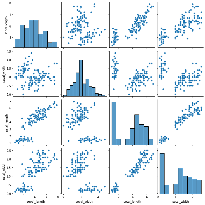
绘制成对的双变量分布

dataset = sns.load_dataset("iris")
dataset.head()

	sepal_length	sepal_width	petal_length	petal_width	species
0	5.1	3.5	1.4	0.2	setosa
1	4.9	3.0	1.4	0.2	setosa
2	4.7	3.2	1.3	0.2	setosa
3	4.6	3.1	1.5	0.2	setosa
4	5.0	3.6	1.4	0.2	setosa

# 斜线上的是数据本身的一个分布，非斜线的是两个变量之间的一个关系
sns.pairplot(dataset)

<seaborn.axisgrid.PairGrid at 0x1f1a0f3f250>

用分类数据绘图

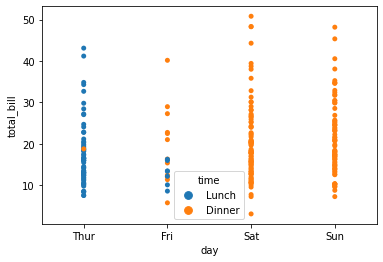
类别散点图

data = sns.load_dataset("tips")

data.head()

	total_bill	tip	sex	smoker	day	time	size
0	16.99	1.01	Female	No	Sun	Dinner	2
1	10.34	1.66	Male	No	Sun	Dinner	3
2	21.01	3.50	Male	No	Sun	Dinner	3
3	23.68	3.31	Male	No	Sun	Dinner	2
4	24.59	3.61	Female	No	Sun	Dinner	4

# (1) x，y，hue：用于绘制长格式数据的输入。hue根据所指定的属性上色分类
# (2) data：用于绘制的数据集。如果x和y不存在，则它将作为宽格式，否则将作为长格式。
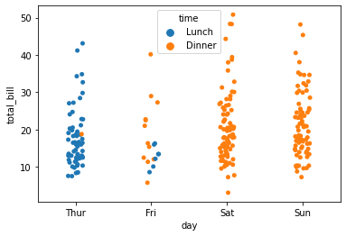
# (3) jitter：表示抖动的程度(仅沿类別轴)。当很多数据点重叠时，可以指定抖动的数量或者设为Tue使用默认值。

sns.stripplot(x="day",y="total_bill",data=data,hue="time",jitter=False)

<AxesSubplot:xlabel='day', ylabel='total_bill'>

sns.stripplot(x="day",y="total_bill",data=data,hue="time",jitter=True)

<AxesSubplot:xlabel='day', ylabel='total_bill'>

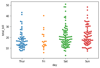
# swarmplot 让所有数据无重合现象
sns.swarmplot(x="day",y="total_bill",data=data)

<AxesSubplot:xlabel='day', ylabel='total_bill'>

类别内数据分布

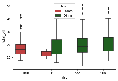
# 箱型图
# (1) palette：用于设置不同级别色相的颜色变量。---- palette=["r","g","b","y"]
# (2) saturation：用于设置数据显示的颜色饱和度。---- 使用小数表示
sns.boxplot(x="day",y="total_bill",data=data,hue="time",palette={"g","r"},saturation=0.5)

<AxesSubplot:xlabel='day', ylabel='total_bill'>

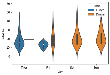
# 绘制小提琴图
sns.violinplot(x="day",y="total_bill",data=data,hue="time")

<AxesSubplot:xlabel='day', ylabel='total_bill'>

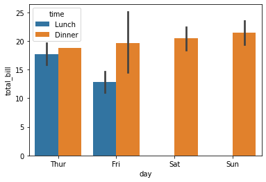
类别内统计估计

sns.barplot(x="day",y="total_bill",data=data,hue="time")

<AxesSubplot:xlabel='day', ylabel='total_bill'>

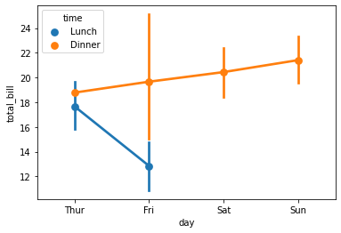
sns.pointplot(x="day",y="total_bill",data=data,hue="time")

<AxesSubplot:xlabel='day', ylabel='total_bill'>

​

​