B站字幕提取

做这个主要是为了提取一些没有翻译的英文公开课的字幕，打印出来便于预习复习。由于技术小白，未能实现全自动化，故按需所取吧。

以数字图像处理【杜克大学】（冈萨雷斯第三版）为例，从视频选集里选择你想要听的那一集，然后把视频的字幕关掉

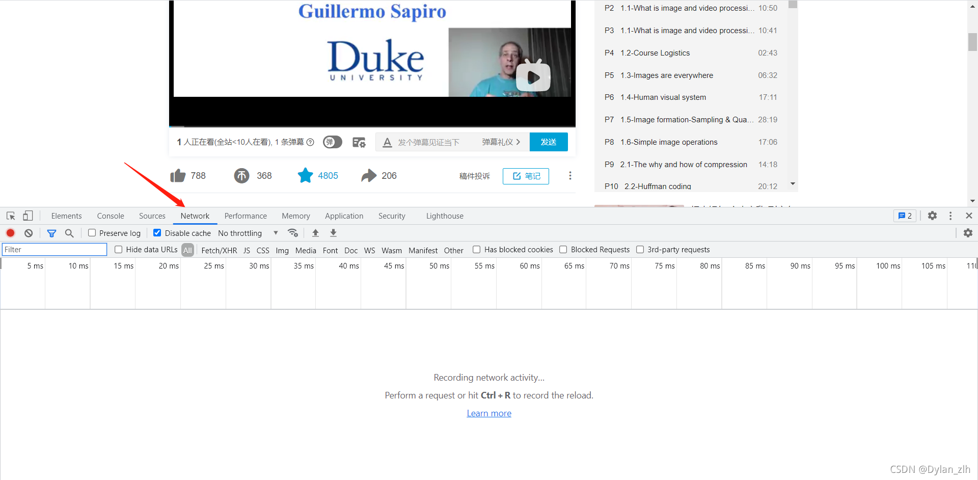
接着，在网页任意地方鼠标右键，选择检查，然后点击Network，如下图

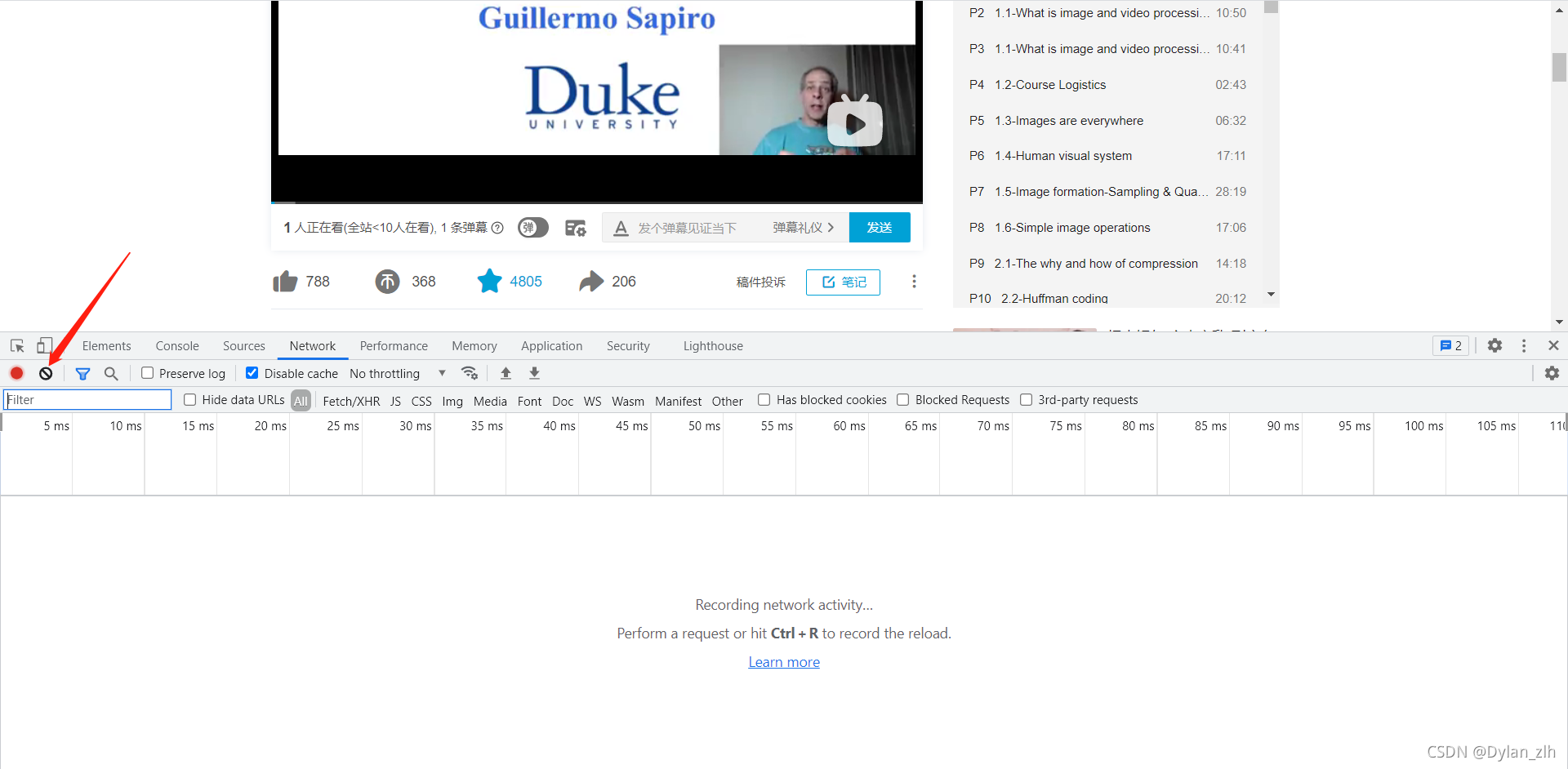
这时刷新一下网页，然后点击clear按钮(便于找到包含字幕的json文件)，再打开字幕，找到json后缀的那一项

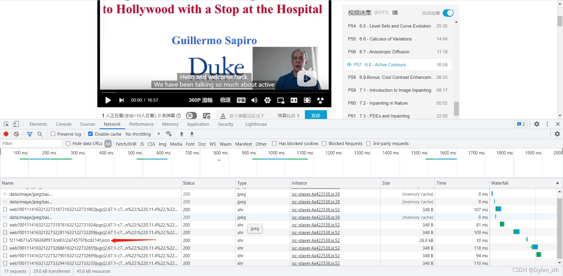
双击json这一项，会重新打开一个网页展示字幕

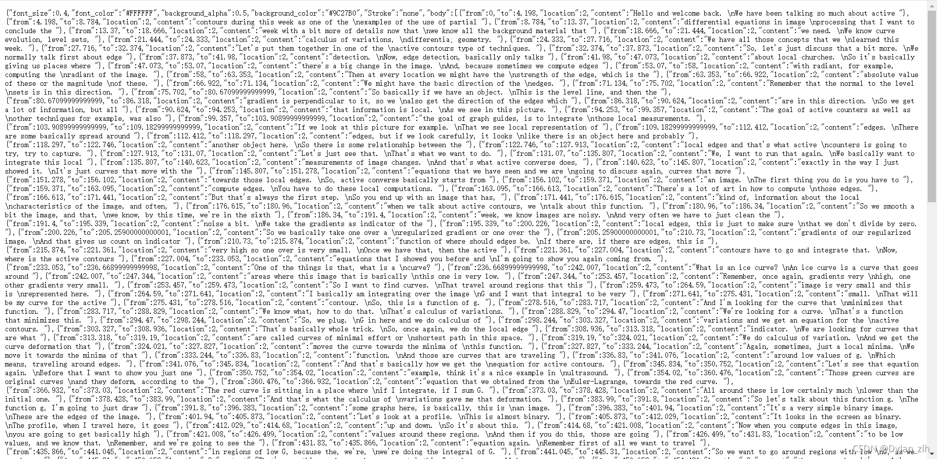
 这是一个字典结构，字幕内容保存在"body"，除了保存字幕内容，还有字幕对应的相应时间段。

提取字幕内容实现如下：

 ①ctrl+A，ctrl+C选择网页的全部内容

②按照结构逻辑提取内容，并保存到文件中

# 将复制的内容保存到变量data中
data = {"font_size":0.4,"font_color":"#FFFFFF","background_alpha":0.5,"background_color":"#9C27B0","Stroke":"none","body":[{"from":0,"to":4.716,"location":2,"content":"Hello and welcome back. \nOne of the fun things of this week is "},{"from":4.716,"to":7.79,"location":2,"content":"that we are learning a lot of background \nmaterial. "},{"from":7.79,"to":12.19,"location":2,"content":"While the background material is \nimportant for image processing, it's "},{"from":12.19,"to":16.91,"location":2,"content":"important for many other disciplines. \nFor example, in the previous video we "},{"from":16.91,"to":20.673,"location":2,"content":"learned about level sets. \nLevel sets are important in image "},{"from":20.673,"to":25.775,"location":2,"content":"processing to the curve evolution like \nactive contours as we have seen numerous "},{"from":25.775,"to":29.156,"location":2,"content":"examples last week. \nWe saw a few this week and we are going "},{"from":29.156,"to":32.09,"location":2,"content":"to see more even in the next coming \nvideos. "},{"from":32.09,"to":37.161,"location":2,"content":"Another topic that is very important in \nmathematics and is also important in "},{"from":37.161,"to":40.257,"location":2,"content":"image processing is the calculus of \nvariations. "},{"from":40.257,"to":44.604,"location":2,"content":"And that's what we're going to be talking \nright now in this video. "},{"from":44.604,"to":49.346,"location":2,"content":"And then in the next video we're going to \nsee an example of that for image "},{"from":49.346,"to":54.12,"location":2,"content":"denoiseing and image enhancement. \nSo what is calculus of variations? "},{"from":54.12,"to":60.234,"location":2,"content":"The idea is very simple, because it's an \nextension of finding extrema of "},{"from":60.234,"to":63.801,"location":2,"content":"functions. \nBut now we are going to be finding "},{"from":63.801,"to":68.047,"location":2,"content":"extrema of functionals. \nAnd what do I mean by that? "},{"from":68.047,"to":71.78999999999999,"location":2,"content":"We're going to have images like you. \nAnd. "},{"from":71.78999999999999,"to":75.75,"location":2,"content":"It's derivatives. \nSo this is going to be an image for us. "},{"from":75.75,"to":80.346,"location":2,"content":"And we're going to be looking at \nminimizing a function of the image. "},{"from":80.346,"to":85.791,"location":2,"content":"Might be the image is square, might be \nthe gradient of the image, might be the "},{"from":85.791,"to":89.751,"location":2,"content":"Laplacian of the image. \nSo we're going to be trying to find "},{"from":89.751,"to":95.338,"location":2,"content":"what's the image that minimizes that \nfunction in the same way that we tried to "},{"from":95.338,"to":99.157,"location":2,"content":"find, what's the point that minimizes a \ngiven function. "},{"from":99.157,"to":104.46000000000001,"location":2,"content":"For example, if I draw this function then \nyou say oh, this is the point that "},{"from":104.46000000000001,"to":108.018,"location":2,"content":"minimizes it. \nBut here, U is by itself what we are "},{"from":108.018,"to":111.755,"location":2,"content":"looking for. \nSo we are not looking for a coordinate, "},{"from":111.755,"to":115.419,"location":2,"content":"we are looking for a function that \nminimizes this. "},{"from":115.419,"to":120.548,"location":2,"content":"This is going to be very clear even in \nthe next slide with an example. "},{"from":120.548,"to":125.458,"location":2,"content":"And we are going to make all the \nconnection of the minimization of "},{"from":125.458,"to":128.829,"location":2,"content":"function X with the minimization of \nfunctions. "},{"from":128.829,"to":134.764,"location":2,"content":"Now, we're going to discuss in a couple \nof minutes that a condition for U to be a "},{"from":134.764,"to":139.373,"location":2,"content":"minimizer of this is to hold. \nThis equation which is called the "},{"from":139.373,"to":145.071,"location":2,"content":"Euler-Lagrange equation and this is the \ntype of partial differential equation "},{"from":145.071,"to":148.65,"location":2,"content":"that we are going to be solving in image \nprocessing. "},{"from":148.65,"to":154.348,"location":2,"content":"Let me illustrate a bit more about this \nand then how we came to this equation "},{"from":154.348,"to":160.04500000000002,"location":2,"content":"which is completely parallel to the \nminimization of regular functions that we "},{"from":160.04500000000002,"to":163.25900000000001,"location":2,"content":"are away from regular standards in \ncalculus. "},{"from":163.25900000000001,"to":168.3,"location":2,"content":"So let's just illustrate, first of all, \nwhat do I mean by a functional. "},{"from":168.3,"to":174.72899999999998,"location":2,"content":"Let's assume that I'm giving two points. \nAnd I am asking you what's the curve "},{"from":174.72899999999998,"to":179.086,"location":2,"content":"connecting these two points that has the \nminimum length. "},{"from":179.086,"to":185,"location":2,"content":"So I am asking you for the function of \nthat curve, the minimizer is going to be "},{"from":185,"to":187.88,"location":2,"content":"a function, not a point. \nThe length of. "},{"from":187.88,"to":193.002,"location":2,"content":"Any curve, absolutely. \nAny curve connecting these two points is "},{"from":193.002,"to":198.042,"location":2,"content":"basically written here. \nThe curve is parameterized as X Ux, we "},{"from":198.042,"to":203.99099999999999,"location":2,"content":"know about that, that's the particular \ncase of that parameterization for "},{"from":203.99099999999999,"to":209.493,"location":2,"content":"basically any curve that goes. \nAnd connect those points. "},{"from":209.493,"to":214.37,"location":2,"content":"the length is. \nAs we know, the derivative of the first "},{"from":214.37,"to":219.94,"location":2,"content":"coordinate squared so that's one squared \nderivative of the second coordinate "},{"from":219.94,"to":222.978,"location":2,"content":"squared. \nSo it's this function that we are going "},{"from":222.978,"to":227.245,"location":2,"content":"to try to optimize. \nWe already know what a function that "},{"from":227.245,"to":231.65699999999998,"location":2,"content":"minimizes the length between two points. \nIt's a straight line. "},{"from":231.65699999999998,"to":236.575,"location":2,"content":"But let's see how we get that. \nYou see calculus offers variations, so "},{"from":236.575,"to":240.12,"location":2,"content":"I'm trying to find U connecting these two \npoints. "},{"from":240.12,"to":247.419,"location":2,"content":"This is the condition for a function to \nbe a minimizer of this function. "},{"from":247.419,"to":252.59,"location":2,"content":"So it's that integral over a function of \nfunctions. "},{"from":252.59,"to":259.39,"location":2,"content":"We haven't arrived at it yet, but we're \ngoing to discuss it in a few slides that "},{"from":259.39,"to":264.235,"location":2,"content":"this is what happened. \nSo F is square root of one plus UX "},{"from":264.235,"to":268.825,"location":2,"content":"squared. \nSo if you just do the numbers and takes, "},{"from":268.825,"to":275.37,"location":2,"content":"you take this and do the derivative \naccording to U minus the derivative that "},{"from":275.37,"to":283.367,"location":2,"content":"is written here, you get this expression. \nSo this expression is nothing else than "},{"from":283.367,"to":291.04,"location":2,"content":"applying this to f as written here. \nNow this equal to zero is a condition for "},{"from":291.04,"to":297.905,"location":2,"content":"the particular U we are looking for to \nsolve the problem that we are searching "},{"from":297.905,"to":303.815,"location":2,"content":"for, meaning the minimizer of the length \nconnecting these two points. "},{"from":303.815,"to":309.03,"location":2,"content":"Now we have this equals zero, the \ndenominator doesn't matter. "},{"from":309.03,"to":315.317,"location":2,"content":"In when we have eight over B equal zero \nwhen its to be equal zero is U, so U "},{"from":315.317,"to":322.1,"location":2,"content":"double derivative equal zero, that means \nthat the first derivative is constant and "},{"from":322.1,"to":327.23,"location":2,"content":"then is that the function is 8X plus B \nthat's a straight line. "},{"from":327.23,"to":332.004,"location":2,"content":"And A and B are found by what's called \nthe boundary conditions. "},{"from":332.004,"to":335.56600000000003,"location":2,"content":"We know that it has to go through these \npoints. "},{"from":335.56600000000003,"to":341.628,"location":2,"content":"So if I replace here X by a zero, I have \nto get this point and if I replace by X "},{"from":341.628,"to":346.1,"location":2,"content":"one, I have to get this point and in that \nway, I get A and B. "},{"from":346.1,"to":352.88,"location":2,"content":"So we see that for length, the function \nthat basically solves the Euler-Lagrange, "},{"from":352.88,"to":357.287,"location":2,"content":"and that's a necessary condition, is a \nstraight line. "},{"from":357.287,"to":363.05,"location":2,"content":"So basically, if we take this curve here, \nit will have certain length. "},{"from":363.05,"to":369.345,"location":2,"content":"But actually, the one that minimizes is \nnot this because this is not a straight "},{"from":369.345,"to":372.533,"location":2,"content":"line. \nThe one that minimizes is this one. "},{"from":372.533,"to":378.75,"location":2,"content":"So, a function to be a minimizer has to \nhaul the Euler-Larange equation. "},{"from":378.75,"to":383.27,"location":2,"content":"Why is that important, and how do we get \nto the Euler-Lagrange equation? "},{"from":383.27,"to":390.065,"location":2,"content":"Let us go for a second back to regular \nfunctions, and how we find the minima of "},{"from":390.065,"to":394.509,"location":2,"content":"a regular function. \nSo you might not remember exactly how we "},{"from":394.509,"to":397.797,"location":2,"content":"do that. \nBut you do remember the result, which is "},{"from":397.797,"to":401.703,"location":2,"content":"going to explain next. \nThe basic idea is, you have a function. "},{"from":401.703,"to":405.06,"location":2,"content":"And you have the function around a \ncertain point. "},{"from":405.06,"to":408.41700000000003,"location":2,"content":"And you do a small perturbation of that \nfunction. "},{"from":408.41700000000003,"to":412.46,"location":2,"content":"And you take the derivative according to \nthat perturbation. "},{"from":412.46,"to":417.872,"location":2,"content":"And the condition for a point to be a \nmaximum or a minimum is that when you do "},{"from":417.872,"to":421.23,"location":2,"content":"any perturbation, the derivative is equal \nto zero. "},{"from":421.23,"to":427.44,"location":2,"content":"If you compute the derivative according \nto the permutation, you get this, and "},{"from":427.44,"to":432.687,"location":2,"content":"this has to hold for every n. \nSo the derivative of the function for "},{"from":432.687,"to":438.365,"location":2,"content":"every end has to be equal zero which \nmeans that this has to be zero, and we "},{"from":438.365,"to":442.227,"location":2,"content":"know that. \nWe know that the condition of a point to "},{"from":442.227,"to":448.057,"location":2,"content":"be an extreme of a function is that it's \nderivative have to be equal to zero. "},{"from":448.057,"to":452.675,"location":2,"content":"Now why is that so important? \nWe know that but why is that so "},{"from":452.675,"to":455.704,"location":2,"content":"important? \nBecause then I can write this "},{"from":455.704,"to":460.216,"location":2,"content":"differential equation. \nXt so I can make X change in the "},{"from":460.216,"to":467.115,"location":2,"content":"direction of minus the derivative and \nthat basically says that you start from a "},{"from":467.115,"to":473.929,"location":2,"content":"point and your next point, because X is \nchanging in time, it just, you move a bit "},{"from":473.929,"to":478.327,"location":2,"content":"in the direction of the derivative of the \nfunction. "},{"from":478.327,"to":484.7,"location":2,"content":"Remember, derivative is tangent so you \nmove a bit to the next spot. "},{"from":484.7,"to":489.283,"location":2,"content":"This is how you move. \nYour next point is this point minus a "},{"from":489.283,"to":492.78,"location":2,"content":"tiny step in the direction of the \nderivative. "},{"from":492.78,"to":498.84,"location":2,"content":"That's what this equation is telling us. \nBecause if we were to discretize this "},{"from":498.84,"to":503.56,"location":2,"content":"equation, we get that, that. \nX. "},{"from":505.54,"to":515.606,"location":2,"content":"We just saw the result there. \nWe had the X at T plus Delta T minus X at "},{"from":515.606,"to":519.63,"location":2,"content":"T. \nDivided by delta T, that's a [INAUDIBLE] "},{"from":519.63,"to":525.9,"location":2,"content":"equation of this. \nThis expression is equal to minus fx and "},{"from":525.9,"to":534.224,"location":2,"content":"that's what we have here so we go slowly. \nIn the direction of the derivative of X "},{"from":534.224,"to":539.054,"location":2,"content":"until we get to this point. \nLet's just see that again. "},{"from":539.054,"to":545.523,"location":2,"content":"We go one step and then we will go \nanother step and another step until "},{"from":545.523,"to":552.084,"location":2,"content":"basically we get to the steady state. \nIn the steady state, we have the XT "},{"from":552.084,"to":556.093,"location":2,"content":"equals zero. \nNothing is changing anymore and, "},{"from":556.093,"to":560.528,"location":2,"content":"therefore, this. \nIs = to zero, which is our condition. "},{"from":560.528,"to":567.016,"location":2,"content":"So once again, we know that the condition \nfor a point to be a minimal of a "},{"from":567.016,"to":571.312,"location":2,"content":"function. \nIs it has to be the derivative = to zero. "},{"from":571.312,"to":576.31,"location":2,"content":"So we take a point. \nI'm going to just show that to you again "},{"from":576.31,"to":581.849,"location":2,"content":"We take a point and we move it in the \ndirection of the derivative and then "},{"from":581.849,"to":587.758,"location":2,"content":"slowly we are moving it in the direction \nof the derivative and we are moving it "},{"from":587.758,"to":592.56,"location":2,"content":"again until it doesn't move anymore. \nWhen it doesn't move anymore. "},{"from":592.56,"to":598.534,"location":2,"content":"This is equal to zero, which is the \ncondition for it to be a minimum. "},{"from":598.534,"to":603.366,"location":2,"content":"So we arrive to a point that is in this \ncase a minimum. "},{"from":603.366,"to":608.55,"location":2,"content":"So this concept extends to functionals, \nin the same fashion. "},{"from":608.55,"to":614.427,"location":2,"content":"Very simple again. \nWe start from a functional, and then "},{"from":614.427,"to":619.93,"location":2,"content":"we're going to ask u to be in extrema, so \nwe do a perturbation. "},{"from":619.93,"to":627.155,"location":2,"content":"So, u is here, the yellow curve. \nIt's basically our original function now. "},{"from":627.155,"to":631.39,"location":2,"content":"We do a perturbation. \nNow, the perturbation, now, is another "},{"from":631.39,"to":634.956,"location":2,"content":"function. \nBecause we're not talking about points. "},{"from":634.956,"to":639.785,"location":2,"content":"We're talking about entire functions. \nSo this is the perturbation. "},{"from":639.785,"to":644.54,"location":2,"content":"And then u tilda is the sum of my \nfunction and the perturbation. "},{"from":644.54,"to":650.63,"location":2,"content":"And what I want is when I replace U by U \ntilde, I replace it by the perturbation "},{"from":650.63,"to":656.341,"location":2,"content":"and I take the derivative, according to \nthe perturbation, has to be equal to "},{"from":656.341,"to":662.203,"location":2,"content":"zero, the same way than when I did the \npoint perturbation for functions, I got "},{"from":662.203,"to":665.553,"location":2,"content":"zero. \nIf I do a function perturbation here, I "},{"from":665.553,"to":669.588,"location":2,"content":"have to get zero. \nFrom this, after a few lines of just "},{"from":669.588,"to":673.7,"location":2,"content":"taking derivatives, we get the \nEuler-Lagrange equation. "},{"from":673.7,"to":679.27,"location":2,"content":"So that's how we get basically the \nEuler-Lagrange equation. "},{"from":679.27,"to":684.65,"location":2,"content":"Doing the derivative according to the \n[INAUDIBLE] that we are using. "},{"from":684.65,"to":690.427,"location":2,"content":"Once you have basically the \nEuler-Lagrange equation, you can do the "},{"from":690.427,"to":695.456,"location":2,"content":"same that we did for functions. \nYou can move your function in the "},{"from":695.456,"to":699.852,"location":2,"content":"direction of the Euler-Lagrange equation \nuntil steady state, "},{"from":699.852,"to":705.613,"location":2,"content":"when you get to state, you have solved \nyour Euler-Lagrange equation. "},{"from":705.613,"to":709.706,"location":2,"content":"So let's just illustrate that here. \nLook what happened. "},{"from":709.706,"to":713.42,"location":2,"content":"I want to put that, basically. \nI want to do that again, "},{"from":713.42,"to":717.233,"location":2,"content":"okay? \nSo you're going to basically move until "},{"from":717.233,"to":723.04,"location":2,"content":"you get to the steady state. \nWhen you get to steady state, basically "},{"from":723.04,"to":727.2,"location":2,"content":"we've got zero. \nSo let us recap what we just saw. "},{"from":727.2,"to":733.784,"location":2,"content":"In regular calculus, we basically are \nmoving a point, not a curve, removing a "},{"from":733.784,"to":740.104,"location":2,"content":"point in the direction of minus the \nderivative and basically we get, the "},{"from":740.104,"to":745.371,"location":2,"content":"solution which is the minima. \nIn the case of the calculus of "},{"from":745.371,"to":752.306,"location":2,"content":"variations, we move, we move the function \nin the direction of the Euler-Lagrange "},{"from":752.306,"to":756.871,"location":2,"content":"basically again the derivative for the \nperturbation. "},{"from":756.871,"to":760.623,"location":2,"content":"We do that all the way to stay state, \nokay? "},{"from":760.623,"to":767.201,"location":2,"content":"And just do that again. \nWe do it all the way to steady state and "},{"from":767.201,"to":772.062,"location":2,"content":"at the point of steady state basically \nthis became zero. "},{"from":772.062,"to":777.937,"location":2,"content":"And we have solved the Euler-Lagrange \nwhich is the condition, basically, for "},{"from":777.937,"to":781.747,"location":2,"content":"getting an extreme amount in this case a \nminima. "},{"from":781.747,"to":785.161,"location":2,"content":"We can change the signs and get the \nmaxima. "},{"from":785.161,"to":790.48,"location":2,"content":"So we are going to see, in the next \nvideo, how we can take you to be an "},{"from":790.48,"to":794.132,"location":2,"content":"image. \nWe'll do some interesting function of F. "},{"from":794.132,"to":799.532,"location":2,"content":"And get, for example. \nBlurring the image or get image noisy. "},{"from":799.532,"to":806.29,"location":2,"content":"So once again, our unknown is the image \nthat basically optimizes this function. "},{"from":806.29,"to":811.622,"location":2,"content":"And we get the complete analogy between \nregular calculus and calculus of "},{"from":811.622,"to":817.54,"location":2,"content":"variations and as I say for [INAUDIBLE] \nand even more for calculus of variations, "},{"from":817.54,"to":821.631,"location":2,"content":"these type of techniques go way beyond \nimage processing. "},{"from":821.631,"to":826.306,"location":2,"content":"What image processing did, and in \nparticular the area of partial "},{"from":826.306,"to":831.347,"location":2,"content":"differential equations, is to borrow \nthese techniques from continuous "},{"from":831.347,"to":835.836,"location":2,"content":"mathematics into this area. \nOnce again, I'm going to show you in the "},{"from":835.836,"to":840.681,"location":2,"content":"next video an example of a function that \nis very useful for image processing. "},{"from":840.681,"to":843.702,"location":2,"content":"I see you in the next video. \nThank you very much."}]}

# 保存到文件
with open('P55.doc','w') as file_object:
    for i in data['body']:
        file_object.write(i['content'])

 这样你想要的那一集字幕就保存到word文档中啦~