matlab：产生脉冲波

夏凉秋落

已于 2023-03-18 19:25:15 修改

阅读量8.6k

点赞数 9

文章标签： matlab

于 2023-03-18 12:10:42 首次发布

本文链接：https://blog.csdn.net/weixin_43778388/article/details/129634889

版权

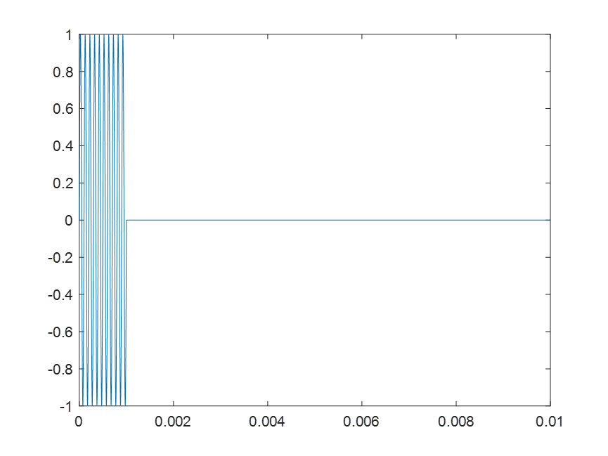
一、matlab产生矩形脉冲

clc;
clear all;
fs = 500e3; %采样率
T=10e-3;    %总时间
pw = 1e-3;  %脉宽
t = 0:1/fs:T;%时间维度
f0=10e3;     %信号的频率
signal=sin(2*pi*f0*t);  
x = rectpuls(t-pw/2,pw).*signal;
plot(t,x);

在这里插入图片描述

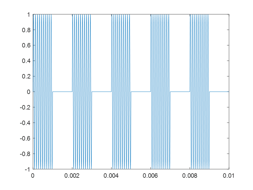
二、 matlab产生矩形脉冲串

matlab产生矩形脉冲串：

figure;
fs=500e3;            %采样率
f0=10e3;             %信号的频率
prf=0.5e3;           %prf
pri=1/prf;           %pri
duty=0.5;            %占空比
pw=duty*pri;          %脉宽
T=10e-3;               %预计总时间
t = 0:1/fs:T;         %总时间维度 
prf_d = 0:1/prf:T;    %脉冲重复周期的时间维度
atten=1.^(1:length(prf_d));   %每个脉冲的衰减值
%采样率，时间维度
D = [prf_d;atten]';                 % prf，脉冲重复周期
Y = pulstran(t-pw/2,D,'rectpuls',pw);          % rectpuls矩形脉冲，以t=0左右开展pw宽度
signal = sin(2*pi*f0.*t);
pulse_signal = signal.*Y;
plot(t,pulse_signal)

在这里插入图片描述

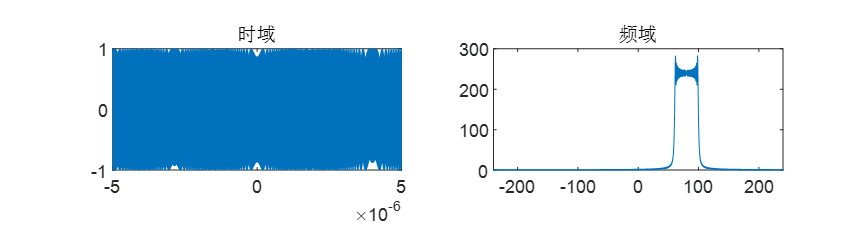
三、matlab产生LFM信号

%% 产生线性调频信号（参考网址https://blog.csdn.net/anwanan8888/article/details/108009366）
B = 40e6;                       %调频带宽
T = 10e-6;                      %脉冲宽度
K = B/T;                        %调频斜率
Fs =480e6;                       %采样频率
F0 = 80e6;                       %发射信号时的瞬时频率，也是信号有效区间发射信号的中心频率
Ts = 1/Fs;                      %采样周期/间隔
N = ceil(T/Ts);                 %采样点数
FFT_Len = 2^nextpow2(2 * N);    %计算FFT的长度
t = linspace(-T/2,T/2,N);
LFM = cos(2 * pi * F0 * t + pi * K * t.^2);
% LFM2 = exp(sqrt(-1) *(2 * pi * F0 * t + pi * K * t.^2));  
figure;
subplot(3,2,1);
plot(t,LFM);
title('时域');
subplot(3,2,2);
f = linspace(-Fs/2,Fs/2,FFT_Len);
LFM_FFT =fftshift(abs(fft(LFM,FFT_Len)));
plot(f/10^6,LFM_FFT);
title('频域');

在这里插入图片描述

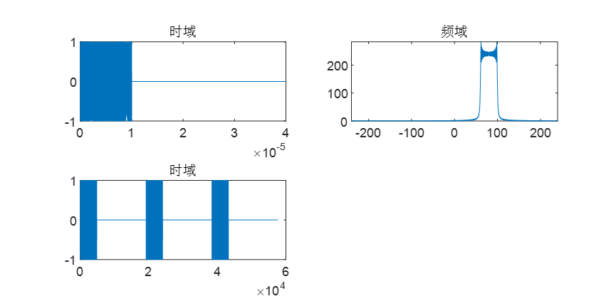
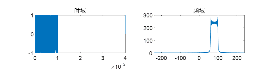
三、matlab产生LFM信号脉冲串

方法一：

%% 产生线性调频信号（参考网址https://blog.csdn.net/anwanan8888/article/details/108009366）
B = 40e6;                       %调频带宽
pw = 10e-6;                      %脉冲宽度
pri=40e-6;                       %重频
K = B/pw;                        %调频斜率
Fs =480e6;                       %采样频率
F0 = 80e6;                       %发射信号时的瞬时频率，也是信号有效区间发射信号的中心频率
Ts = 1/Fs;                      %采样周期/间隔
t=0:Ts:pri;
N = length(t);                 %采样点数
FFT_Len = 2^nextpow2(2 * N);    %计算FFT的长度
delay=0;                        %回波的延时
LFM = rectpuls(t-pw/2-delay,pw).*exp(sqrt(-1) *(2 * pi * F0 *( t-pw/2-delay) + pi * K * (t-pw/2-delay).^2));  
figure;
subplot(3,2,1); 
plot(t,LFM);
title('时域');
subplot(3,2,2);
f = linspace(-Fs/2,Fs/2,FFT_Len);
LFM_FFT =fftshift(abs(fft(LFM,FFT_Len)));
plot(f/10^6,LFM_FFT);
title('频域');
%% 方法一
t=t*M;
M=3;  %脉冲串数目
LFM_plus = repmat(LFM,1,M);
subplot(3,2,3); 
plot(1:length(LFM_plus),LFM_plus);
title('时域');

在这里插入图片描述
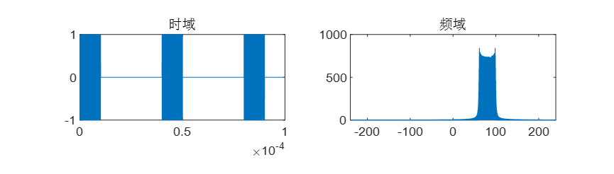
方法二（可以设置任意长度，更倾向这种）：

%% 产生线性调频信号（参考网址https://blog.csdn.net/anwanan8888/article/details/108009366）
B = 40e6;                       %调频带宽
pw = 10e-6;                      %脉冲宽度
pri=40e-6;                       %重频
K = B/pw;                        %调频斜率
Fs =480e6;                       %采样频率
F0 = 80e6;                       %发射信号时的瞬时频率，也是信号有效区间发射信号的中心频率
Ts = 1/Fs;                      %采样周期/间隔
T=100e-6;                        % 总时间
t=0:Ts:T;                       %快时间维
N = length(t);                 %采样点数
FFT_Len = 2^nextpow2(2 * N);    %计算FFT的长度
delay=0;                        %回波的延时
pri_t = 0:pri:T;         %慢时间维
LFM = zeros(1,N);
for ii=1:length(pri_t)
      LFM =LFM+ rectpuls(t-pw/2-delay-pri_t(1,ii),pw).*exp(sqrt(-1) *(2 * pi * F0 *( t-pw/2-delay-pri_t(1,ii)) + pi * K * (t-pw/2-delay-pri_t(1,ii)).^2)); 
end
figure;
subplot(3,2,1); 
plot(t,LFM);
title('时域');
subplot(3,2,2);
f = linspace(-Fs/2,Fs/2,FFT_Len);
LFM_FFT =fftshift(abs(fft(LFM,FFT_Len)));
plot(f/10^6,LFM_FFT);
title('频域');