


(一)图像的平滑滤波
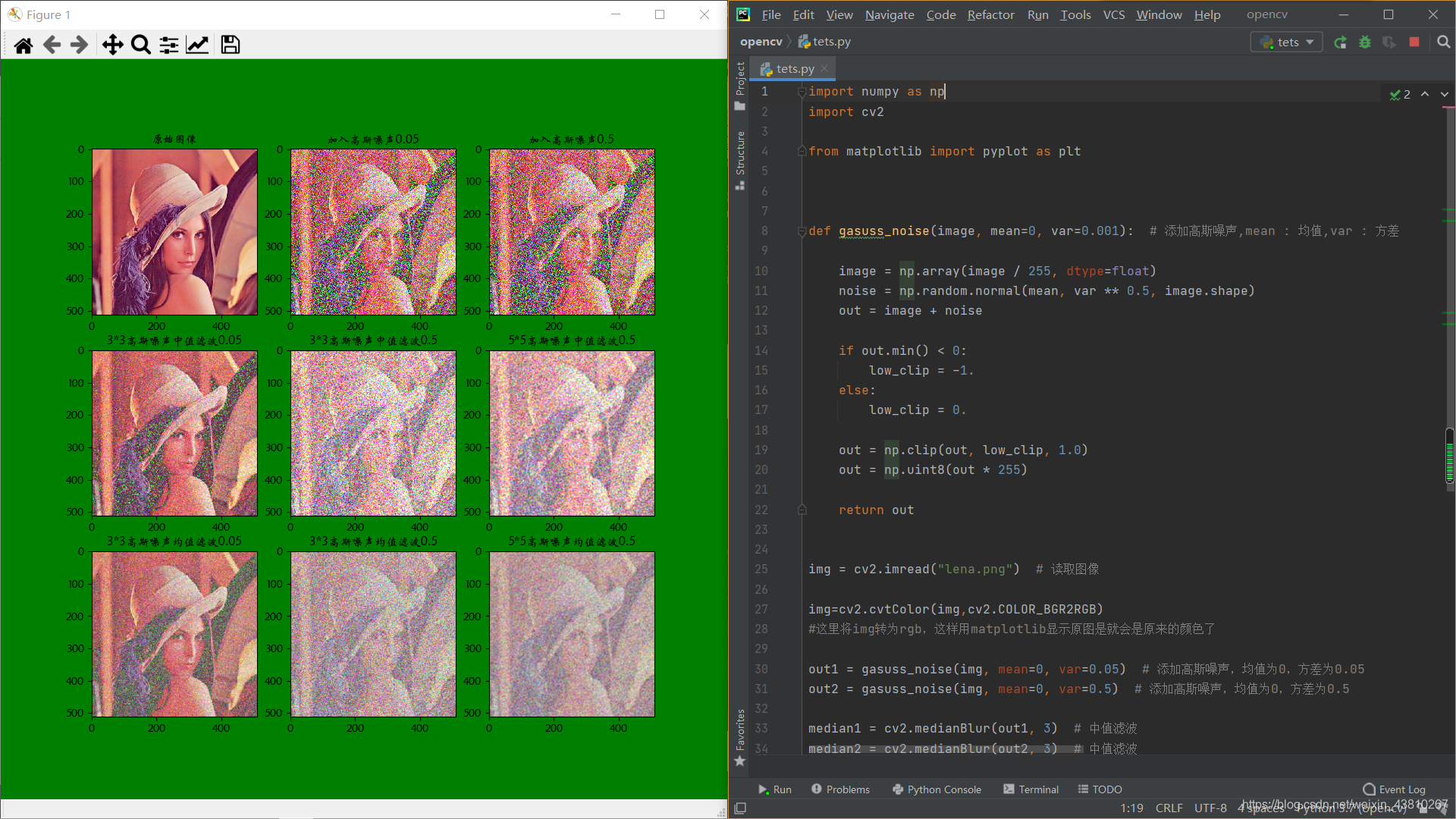
平滑与锐化相反, 就是滤掉高频分量, 从而达到减少图象噪声, 使图片变得有些模糊。 因此又称为低通滤波。均值滤波和和中值滤波的对比均值滤波和和中值滤波都可以起到平滑图像, 虑去噪声的功能。 均值滤波采用线性的方法, 平均整个窗口范围内的像素值, 均值滤波本身存在着固有的缺陷,即它不能很好地保护图像细节, 在图像去噪的同时也破坏了图像的细节部分,从而使图像变得模糊, 不能很好地去除噪声点。 均值滤波对高斯噪声表现较好, 对椒盐噪声表现较差。 中值滤波采用非线性的方法, 它在平滑脉冲噪声方面非常有效,同时它可以保护图像尖锐的边缘, 选择适当的点来替代污染点的值, 所以处理效果好, 对椒盐噪声表现较好, 对高斯噪声表现较差
这里使用opencv的内置函数,中值滤波和均值滤波函数对图像进行平滑处理,分别用33和55的卷积核,使用cv2.medianBlur(均值滤波函数)和cv2.Blur(中值滤波函数)函数对方差不同的高斯噪声图像进行平滑滤波处理、
代码如下:(下面是对彩色图像进行处理)
import numpy as np
import cv2

from matplotlib import pyplot as plt


def gasuss_noise(image, mean=0, var=0.001):  # 添加高斯噪声,mean : 均值,var : 方差

    image = np.array(image / 255, dtype=float)
    noise = np.random.normal(mean, var ** 0.5, image.shape)
    out = image + noise

    if out.min() < 0:
        low_clip = -1.
    else:
        low_clip = 0.

    out = np.clip(out, low_clip, 1.0)
    out = np.uint8(out * 255)

    return out


img = cv2.imread("lena.png")  # 读取图像

img=cv2.cvtColor(img,cv2.COLOR_BGR2RGB)
#这里将img转为rgb,这样用matplotlib显示原图是就会是原来的颜色了

out1 = gasuss_noise(img, mean=0, var=0.05)  # 添加高斯噪声,均值为0,方差为0.05
out2 = gasuss_noise(img, mean=0, var=0.5)  # 添加高斯噪声,均值为0,方差为0.5

median1 = cv2.medianBlur(out1, 3)  # 中值滤波
median2 = cv2.medianBlur(out2, 3)  # 中值滤波
median3 = cv2.medianBlur(out2, 5)  # 中值滤波

blur1 = cv2.blur(out1, (3, 3))
blur2 = cv2.blur(out2, (3, 3))
blur3 = cv2.blur(out2, (5, 5))

plt.figure(figsize=(11, 10), facecolor='green')  # 创建figure
plt.rcParams['font.sans-serif'] = 'STXINWEI'  # 设置中文字体为华文新魏

titles = ['原始图像', '加入高斯噪声0.05','加入高斯噪声0.5', '3*3高斯噪声中值滤波0.05', '3*3高斯噪声中值滤波0.5', '5*5高斯噪声中值滤波0.5', '3*3高斯噪声均值滤波0.05','3*3高斯噪声均值滤波0.5','5*5高斯噪声均值滤波0.5']
images = [img, out1, out1, median1, median2, median3,blur1,blur2,blur3]

for i in range(9):
    plt.subplot(3, 3, i + 1), plt.imshow(images[i])
    plt.title(titles[i], fontsize=11)

plt.show()
效果如下
代码如下:(下面是对灰度图像进行处理)
import numpy as np
import cv2

from matplotlib import pyplot as plt


def gasuss_noise(image, mean=0, var=0.001):  # 添加高斯噪声,mean : 均值,var : 方差

    image = np.array(image / 255, dtype=float)
    noise = np.random.normal(mean, var ** 0.5, image.shape)
    out = image + noise

    if out.min() < 0:
        low_clip = -1.
    else:
        low_clip = 0.

    out = np.clip(out, low_clip, 1.0)
    out = np.uint8(out * 255)

    return out


img = cv2.imread("lena.png",0)  # 读取图像

#img=cv2.cvtColor(img,cv2.COLOR_BGR2RGB)
#这里将img转为rgb,这样用matplotlib显示原图是就会是原来的颜色了

out1 = gasuss_noise(img, mean=0, var=0.05)  # 添加高斯噪声,均值为0,方差为0.05
out2 = gasuss_noise(img, mean=0, var=0.5)  # 添加高斯噪声,均值为0,方差为0.5

median1 = cv2.medianBlur(out1, 3)  # 中值滤波
median2 = cv2.medianBlur(out2, 3)  # 中值滤波
median3 = cv2.medianBlur(out2, 5)  # 中值滤波

blur1 = cv2.blur(out1, (3, 3))
blur2 = cv2.blur(out2, (3, 3))
blur3 = cv2.blur(out2, (5, 5))

plt.figure(figsize=(11, 10), facecolor='green')  # 创建figure
plt.rcParams['font.sans-serif'] = 'STXINWEI'  # 设置中文字体为华文新魏

titles = ['原始图像', '加入高斯噪声0.05','加入高斯噪声0.5', '3*3高斯噪声中值滤波0.05', '3*3高斯噪声中值滤波0.5', '5*5高斯噪声中值滤波0.5', '3*3高斯噪声均值滤波0.05','3*3高斯噪声均值滤波0.5','5*5高斯噪声均值滤波0.5']
images = [img, out1, out1, median1, median2, median3,blur1,blur2,blur3]

for i in range(9):
    plt.subplot(3, 3, i + 1), plt.imshow(images[i],'gray')
    plt.title(titles[i], fontsize=11)

plt.show()
效果如下
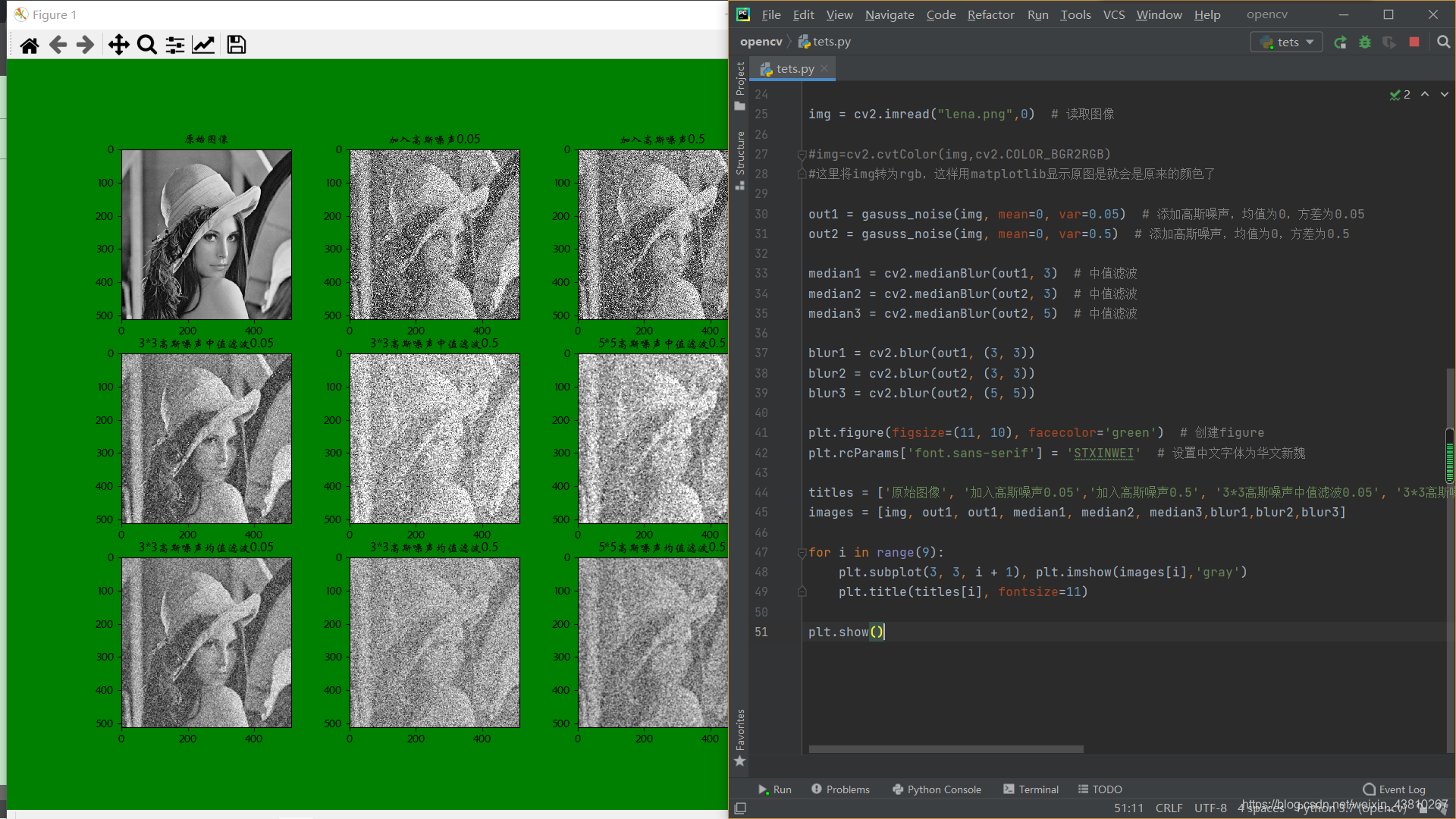
PS:对彩色图像和灰度图像处理的代码大致相同,但因为我是使用opencv读取的图像(opencv读取后的彩色图像格式为BGR),matplotlib显示的图像(matplotlib只有正常显示RGB的彩色图像),所以在上面处理彩色图像的代码中,img=cv2.cvtColor(img,cv2.COLOR_BGR2RGB),进行转换。灰度图就不用管了
(二)图像的锐化滤波之拉普拉斯算子
锐化滤波器:增强被模糊的细节,减弱或消除图像中的低频率分量, 但不影响高频率分量。低频分量对应图像中灰度值缓慢变化的区域,锐化滤波器将这些分量滤去,可使图像反差增加,边缘明显
锐化通过增强高频分量来减少图象中的模糊,因此又称为高通滤波。 锐化处理在增强图象边缘的同时增加了图象的噪声
使用锐化滤波器对高斯噪声分别对彩色图像和灰度图像进行处理,用numpy数组分别生成拉普拉斯算子,普瑞斯特算子,索贝尔算子对图像进行滤波处理
只需要将不同的算子传入cv2.filter2D()函数
cv2.filter2D(src, ddepth, kernel[, dst[, anchor[, delta[, borderType]]]])
| 参数 | 解释 |
|---|---|
| src | 输入图像 |
| ddepth | 目标图像的所需深度,一般为-1,表示输出图像与原图像有相同的深度 |
| kernel | 卷积核(或相当于相关核),单通道浮点矩阵;如果要将不同的内核应用于不同的通道,请使用拆分将图像拆分为单独的颜色平面,然后单独处理它们。 |
| anchor | 内核的锚点,指示内核中过滤点的相对位置;锚应位于内核中;默认值(-1,-1)表示锚位于内核中心。 |
| detal | 在将它们存储在dst中之前,将可选值添加到已过滤的像素中。类似于偏置。 |
| borderType | 像素外推法,参见BorderTypes |
下面是使用不同的拉普拉斯算子对彩色图像进行锐化处理
看看代码吧:
import numpy as np
import cv2
from matplotlib import pyplot as plt


img = cv2.imread("lena.png")  # 读取图像

img=cv2.cvtColor(img,cv2.COLOR_BGR2RGB)
#这里将img转为rgb,这样用matplotlib显示原图是就会是原来的颜色了

l0 = np.array([[0, 1, 0]  , [1, -4, 1],  [0, 1, 0]]) #定义了卷积核,对每一个像素进行操作
l1 = np.array([[-1,-1, -1], [-1, 8, -1], [-1,-1, -1]])
l2 = np.array([[-1,-1, -1], [-1,9, -1],  [-1,-1, -1]])
l3 = np.array([[-1,-1, -1], [-1,10, -1], [-1,-1, -1]])/2
l4 = np.array([[-1,-1, -1], [-1,11, -1], [-1,-1, -1]])/3

dst_l0 = cv2.filter2D(img, -1, l0)
dst_l1 = cv2.filter2D(img, -1, l1)
dst_l2 = cv2.filter2D(img, -1, l2)
dst_l3 = cv2.filter2D(img, -1, l3)
dst_l4 = cv2.filter2D(img, -1, l4)


plt.figure(figsize=(11, 10), facecolor='green')  # 创建figure
plt.rcParams['font.sans-serif'] = 'STXINWEI'  # 设置中文字体为华文新魏

titles = ['原始图像', 'LaplacianL0','LaplacianL1', 'LaplacianL2', 'LaplacianL3', 'LaplacianL4']
images = [img, dst_l0, dst_l1, dst_l2, dst_l3, dst_l4]

for i in range(6):
    plt.subplot(2, 3, i + 1), plt.imshow(images[i])
    plt.title(titles[i], fontsize=11)

plt.show()
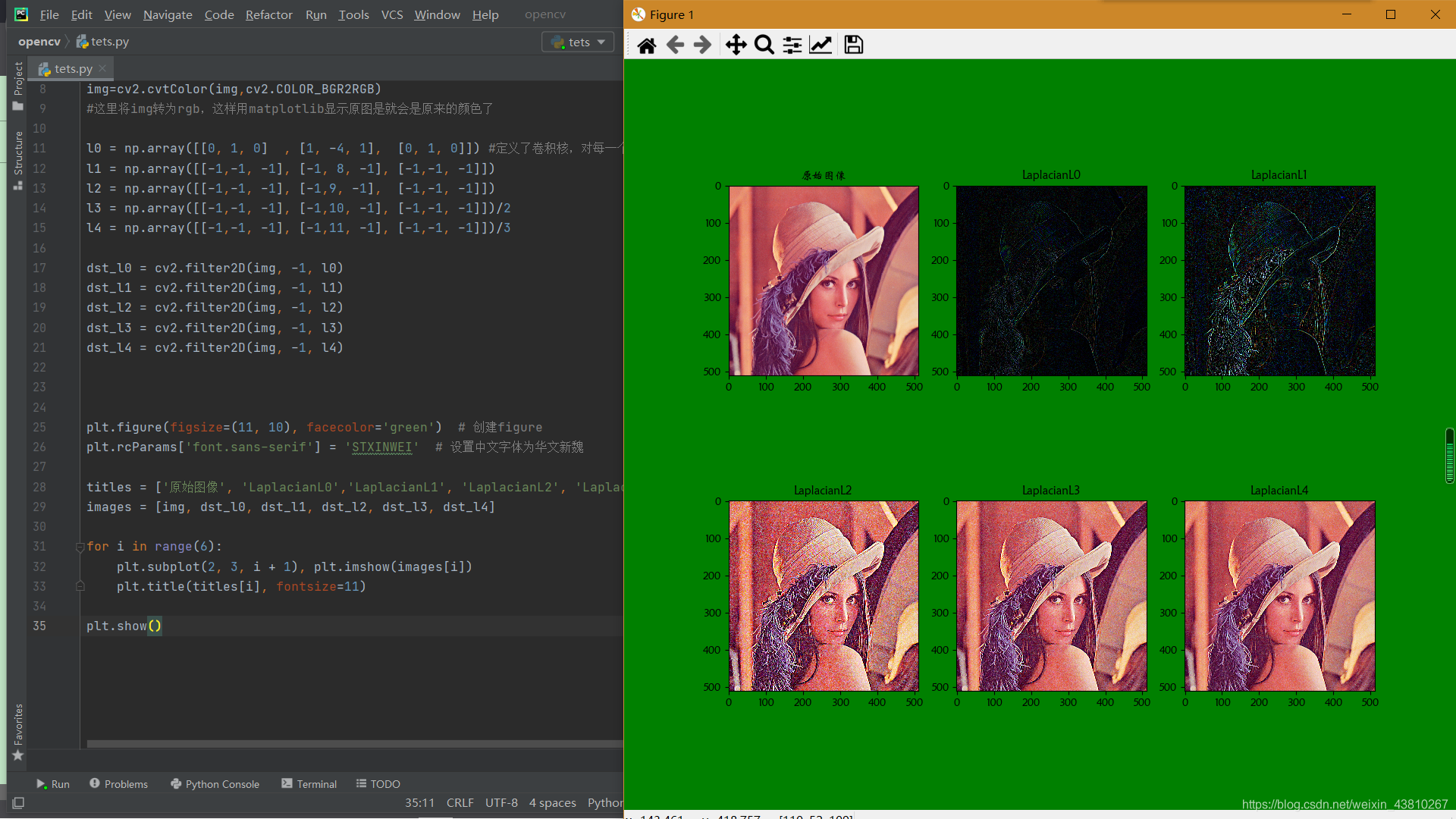
效果如上图,上面是对彩色图像进行处理。
下面是对灰度图像进行处理,代码如下:
import numpy as np
import cv2
from matplotlib import pyplot as plt


img = cv2.imread("lena.png",0)  # 读取图像


l0 = np.array([[0, 1, 0]  , [1, -4, 1],  [0, 1, 0]]) #定义了卷积核,对每一个像素进行操作
l1 = np.array([[-1,-1, -1], [-1, 8, -1], [-1,-1, -1]])
l2 = np.array([[-1,-1, -1], [-1,9, -1],  [-1,-1, -1]])
l3 = np.array([[-1,-1, -1], [-1,10, -1], [-1,-1, -1]])/2
l4 = np.array([[-1,-1, -1], [-1,11, -1], [-1,-1, -1]])/3

dst_l0 = cv2.filter2D(img, -1, l0)
dst_l1 = cv2.filter2D(img, -1, l1)
dst_l2 = cv2.filter2D(img, -1, l2)
dst_l3 = cv2.filter2D(img, -1, l3)
dst_l4 = cv2.filter2D(img, -1, l4)


plt.figure(figsize=(11, 10), facecolor='green')  # 创建figure
plt.rcParams['font.sans-serif'] = 'STXINWEI'  # 设置中文字体为华文新魏

titles = ['原始图像', 'LaplacianL0','LaplacianL1', 'LaplacianL2', 'LaplacianL3', 'LaplacianL4']
images = [img, dst_l0, dst_l1, dst_l2, dst_l3, dst_l4]

for i in range(6):
    plt.subplot(2, 3, i + 1), plt.imshow(images[i],'gray')
    plt.title(titles[i], fontsize=11)

plt.show()
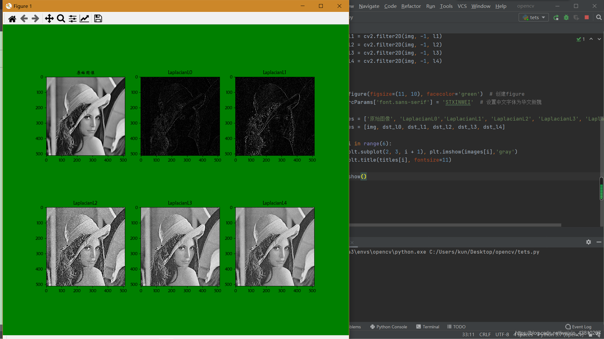
灰度图的处理效果如上
(三)图像的锐化滤波之普瑞斯特算子与索贝尔算子
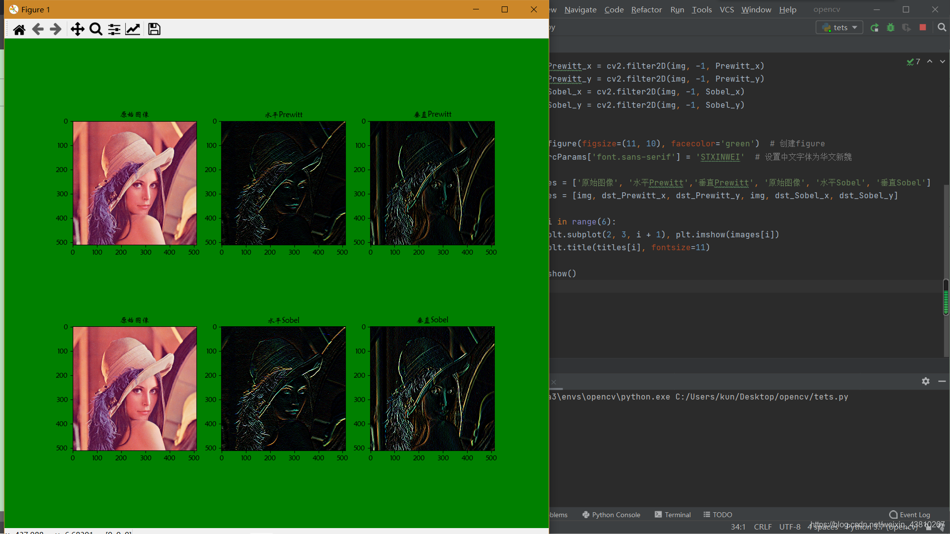
下面分别使用普瑞斯特算子与索贝尔算子对彩色图像进行处理
import numpy as np
import cv2
from matplotlib import pyplot as plt


img = cv2.imread("lena.png")  # 读取图像

img=cv2.cvtColor(img,cv2.COLOR_BGR2RGB)
#这里将img转为rgb,这样用matplotlib显示原图是就会是原来的颜色了

Prewitt_x = np.array([[1,1,1],[0,0,0],[-1,-1,-1]]) #定义了卷积核,对每一个像素进行操作
Prewitt_y = np.array([[-1,0,1],[-1,0,1],[-1,0,1]])
Sobel_x = np.array([[1,2,1],[0,0,0],[-1,-2,-1]])
Sobel_y = np.array([[-1,0,1],[-2,0,2],[-1,0,1]])


dst_Prewitt_x = cv2.filter2D(img, -1, Prewitt_x)
dst_Prewitt_y = cv2.filter2D(img, -1, Prewitt_y)
dst_Sobel_x = cv2.filter2D(img, -1, Sobel_x)
dst_Sobel_y = cv2.filter2D(img, -1, Sobel_y)


plt.figure(figsize=(11, 10), facecolor='green')  # 创建figure
plt.rcParams['font.sans-serif'] = 'STXINWEI'  # 设置中文字体为华文新魏

titles = ['原始图像', '水平Prewitt','垂直Prewitt', '原始图像', '水平Sobel', '垂直Sobel']
images = [img, dst_Prewitt_x, dst_Prewitt_y, img, dst_Sobel_x, dst_Sobel_y]

for i in range(6):
    plt.subplot(2, 3, i + 1), plt.imshow(images[i])
    plt.title(titles[i], fontsize=11)

plt.show()
效果如下:
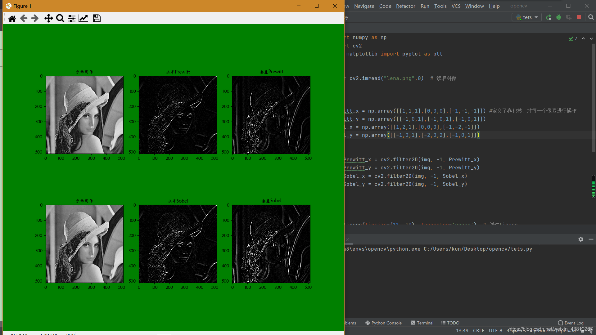
下面分别使用普瑞斯特算子与索贝尔算子对灰度图像图像进行处理
import numpy as np
import cv2
from matplotlib import pyplot as plt


img = cv2.imread("lena.png",0)  # 读取图像


Prewitt_x = np.array([[1,1,1],[0,0,0],[-1,-1,-1]]) #定义了卷积核,对每一个像素进行操作
Prewitt_y = np.array([[-1,0,1],[-1,0,1],[-1,0,1]])
Sobel_x = np.array([[1,2,1],[0,0,0],[-1,-2,-1]])
Sobel_y = np.array([[-1,0,1],[-2,0,2],[-1,0,1]])


dst_Prewitt_x = cv2.filter2D(img, -1, Prewitt_x)
dst_Prewitt_y = cv2.filter2D(img, -1, Prewitt_y)
dst_Sobel_x = cv2.filter2D(img, -1, Sobel_x)
dst_Sobel_y = cv2.filter2D(img, -1, Sobel_y)


plt.figure(figsize=(11, 10), facecolor='green')  # 创建figure
plt.rcParams['font.sans-serif'] = 'STXINWEI'  # 设置中文字体为华文新魏

titles = ['原始图像', '水平Prewitt','垂直Prewitt', '原始图像', '水平Sobel', '垂直Sobel']
images = [img, dst_Prewitt_x, dst_Prewitt_y, img, dst_Sobel_x, dst_Sobel_y]

for i in range(6):
    plt.subplot(2, 3, i + 1), plt.imshow(images[i],'gray')
    plt.title(titles[i], fontsize=11)

plt.show()
(四)结语
木有了
如果有什么错误的地方,还请大家批评指正,最后,希望小伙伴们都能有所收获。


 1460
1460


 被折叠的 条评论
为什么被折叠?
被折叠的 条评论
为什么被折叠?
 到【灌水乐园】发言


