


1、基础矩阵原理
如果已知基础矩阵F,以及一个3D点在一个像面上的像素坐标p,则可以求得在另一个像面上的像素坐标p‘。这个是基础矩阵的作用,可以表征两个相机的相对位置及相机内参数。

设X在C,C’坐标系中的相对坐标分别p,p’,则有

根据:
其中:

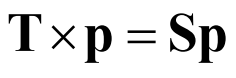
推得:

其中的RS相乘得到的E即为本质矩阵,描述了空间中的点在两个坐标系中的坐标对应关系。
根据前述, K 和 K’ 分别为两个相机的内参矩阵,有:
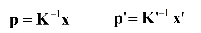

其中的F即为基础矩阵,描述了空间中的点在两个像平面中的坐标对应关系。
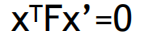
基础矩阵是对极几何的代数表达方式,描述了图像中任意对应点 x↔x’ 之间的约束关系。F 为 3x3 矩阵,秩为2,对任意匹配点对 x↔x’ 均满足:
基础矩阵的两大作用是简化匹配去除错配特征。
2、代码实现SFM的特征提取与匹配
首先是求两张图的基础矩阵
代码如下:
#!/usr/bin/env python
# coding: utf-8

# In[1]:
from PIL import Image
from numpy import *
from pylab import *
import numpy as np
from imp import reload


# In[2]:
import importlib
from PCV.geometry import camera
from PCV.geometry import homography
from PCV.geometry import sfm
from PCV.localdescriptors import sift

camera = importlib.reload(camera)
homography = importlib.reload(homography)
sfm = importlib.reload(sfm)
sift =importlib.reload(sift)


# In[3]:


# Read features
im1 = array(Image.open('image5/1.jpg'))
sift.process_image('image5/1.jpg', 'im1.sift')
l1, d1 = sift.read_features_from_file('im1.sift')

im2 = array(Image.open('image5/2.jpg'))
sift.process_image('image5/2.jpg', 'im2.sift')
l2, d2 = sift.read_features_from_file('im2.sift')


# In[9]:


matches = sift.match_twosided(d1, d2)


# In[10]:


ndx = matches.nonzero()[0]
x1 = homography.make_homog(l1[ndx, :2].T)
ndx2 = [int(matches[i]) for i in ndx]
x2 = homography.make_homog(l2[ndx2, :2].T)

x1n = x1.copy()
x2n = x2.copy()


# In[11]:


print (len(ndx))


# In[12]:


figure(figsize=(16,16))
sift.plot_matches(im1, im2, l1, l2, matches, True)
show()


# In[13]:


# Chapter 5 Exercise 1
# Don't use K1, and K2

#def F_from_ransac(x1, x2, model, maxiter=5000, match_threshold=1e-6):
def F_from_ransac(x1, x2, model, maxiter=5000, match_threshold=1e-6):
    """ Robust estimation of a fundamental matrix F from point
    correspondences using RANSAC (ransac.py from
    http://www.scipy.org/Cookbook/RANSAC).

    input: x1, x2 (3*n arrays) points in hom. coordinates. """

    from PCV.tools import ransac
    data = np.vstack((x1, x2))
    d = 20 # 20 is the original
    # compute F and return with inlier index
    F, ransac_data = ransac.ransac(data.T, model,8, maxiter, match_threshold, d, return_all=True)
    return F, ransac_data['inliers']


# In[15]:


# find E through RANSAC
model = sfm.RansacModel()
F, inliers = F_from_ransac(x1n, x2n, model, maxiter=5000, match_threshold=1e-3)


# In[16]:


print (len(x1n[0]))
print (len(inliers))


# In[17]:


P1 = array([[1, 0, 0, 0], [0, 1, 0, 0], [0, 0, 1, 0]])
P2 = sfm.compute_P_from_fundamental(F)


# In[18]:


# triangulate inliers and remove points not in front of both cameras
X = sfm.triangulate(x1n[:, inliers], x2n[:, inliers], P1, P2)


# In[19]:


# plot the projection of X
cam1 = camera.Camera(P1)
cam2 = camera.Camera(P2)
x1p = cam1.project(X)
x2p = cam2.project(X)


# In[20]:


figure()
imshow(im1)
gray()
plot(x1p[0], x1p[1], 'o')
#plot(x1[0], x1[1], 'r.')
axis('off')

figure()
imshow(im2)
gray()
plot(x2p[0], x2p[1], 'o')
#plot(x2[0], x2[1], 'r.')
axis('off')
show()


# In[21]:


figure(figsize=(16, 16))
im3 = sift.appendimages(im1, im2)
im3 = vstack((im3, im3))

imshow(im3)

cols1 = im1.shape[1]
rows1 = im1.shape[0]
for i in range(len(x1p[0])):
    if (0<= x1p[0][i]<cols1) and (0<= x2p[0][i]<cols1) and (0<=x1p[1][i]<rows1) and (0<=x2p[1][i]<rows1):
        plot([x1p[0][i], x2p[0][i]+cols1],[x1p[1][i], x2p[1][i]],'c')
axis('off')
show()


# In[22]:


print (F)


# In[23]:


# Chapter 5 Exercise 2

x1e = []
x2e = []
ers = []
for i,m in enumerate(matches):
    if m>0: #plot([locs1[i][0],locs2[m][0]+cols1],[locs1[i][1],locs2[m][1]],'c')

        p1 = array([l1[i][0], l1[i][1], 1])
        p2 = array([l2[m][0], l2[m][1], 1])


        # Use Sampson distance as error
        Fx1 = dot(F, p1)
        Fx2 = dot(F, p2)
        denom = Fx1[0]**2 + Fx1[1]**2 + Fx2[0]**2 + Fx2[1]**2
        e = (dot(p1.T, dot(F, p2)))**2 / denom
        x1e.append([p1[0], p1[1]])
        x2e.append([p2[0], p2[1]])
        ers.append(e)
x1e = array(x1e)
x2e = array(x2e)
ers = array(ers)


# In[24]:


indices = np.argsort(ers)
x1s = x1e[indices]
x2s = x2e[indices]
ers = ers[indices]
x1s = x1s[:20]
x2s = x2s[:20]


# In[25]:


figure(figsize=(16, 16))
im3 = sift.appendimages(im1, im2)
im3 = vstack((im3, im3))

imshow(im3)

cols1 = im1.shape[1]
rows1 = im1.shape[0]
for i in range(len(x1s)):
    if (0<= x1s[i][0]<cols1) and (0<= x2s[i][0]<cols1) and (0<=x1s[i][1]<rows1) and (0<=x2s[i][1]<rows1):
        plot([x1s[i][0], x2s[i][0]+cols1],[x1s[i][1], x2s[i][1]],'c')
axis('off')
show()


# In[ ]:
1. 室内
sift特征匹配结果如下:

得到的基础矩阵为:
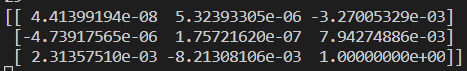
恢复这些点的三维位置:


修改特征匹配结果后:

2. 室外
两张图分别是:左边的为远点,右边的为近点拍摄的中山纪念馆
sift特征匹配结果如下:

得到的基础矩阵为:
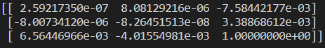
恢复这些点的三维位置:


修改特征匹配结果后:

结果分析:
可以看出来室内由于场景复杂,匹配的特征点更精确一些。而室外由于建筑物存在多处相似特征点导致部分匹配出现错误。但是室内部分的实验是挑了一个结果比较好的展示的,在多次取材过程中,恢复点的三维位置时出现了下图这种奇怪的点位置…好像修改阈值即可,原素材删除了所以无法重新实验。

三维点和照相机矩阵
算法使用的是八点算法,代码如下:
# coding: utf-8

# In[1]:

from PIL import Image
from numpy import *
from pylab import *
import numpy as np
import importlib


# In[2]:

from PCV.geometry import camera
from PCV.geometry import homography
from PCV.geometry import sfm
from PCV.localdescriptors import sift
camera = importlib.reload(camera)
homography = importlib.reload(homography)
sfm = importlib.reload(sfm)
sift =importlib.reload(sift)


# In[3]:

# Read features
im1 = array(Image.open('image5/1.jpg'))
sift.process_image('image5/1.jpg', 'im1.sift')

im2 = array(Image.open('image5/2.jpg'))
sift.process_image('image5/2.jpg', 'im2.sift')


# In[4]:

l1, d1 = sift.read_features_from_file('im1.sift')
l2, d2 = sift.read_features_from_file('im2.sift')


# In[5]:

matches = sift.match_twosided(d1, d2)


# In[6]:

ndx = matches.nonzero()[0]
x1 = homography.make_homog(l1[ndx, :2].T)
ndx2 = [int(matches[i]) for i in ndx]
x2 = homography.make_homog(l2[ndx2, :2].T)

d1n = d1[ndx]
d2n = d2[ndx2]
x1n = x1.copy()
x2n = x2.copy()


# In[7]:

figure(figsize=(16,16))
sift.plot_matches(im1, im2, l1, l2, matches, True)
show()


# In[26]:

#def F_from_ransac(x1, x2, model, maxiter=5000, match_threshold=1e-6):
def F_from_ransac(x1, x2, model, maxiter=5000, match_threshold=1e-6):
    """ Robust estimation of a fundamental matrix F from point
    correspondences using RANSAC (ransac.py from
    http://www.scipy.org/Cookbook/RANSAC).

    input: x1, x2 (3*n arrays) points in hom. coordinates. """

    from PCV.tools import ransac
    data = np.vstack((x1, x2))
    d = 10 # 20 is the original
    # compute F and return with inlier index
    F, ransac_data = ransac.ransac(data.T, model,
                                   8, maxiter, match_threshold, d, return_all=True)
    return F, ransac_data['inliers']


# In[27]:

# find F through RANSAC
model = sfm.RansacModel()
F, inliers = F_from_ransac(x1n, x2n, model, maxiter=5000, match_threshold=1e-5)
print (F)


# In[28]:

P1 = array([[1, 0, 0, 0], [0, 1, 0, 0], [0, 0, 1, 0]])
P2 = sfm.compute_P_from_fundamental(F)


# In[29]:

print (P2)
print (F)


# In[30]:

# P2, F (1e-4, d=20)
# [[ -1.48067422e+00   1.14802177e+01   5.62878044e+02   4.74418238e+03]
#  [  1.24802182e+01  -9.67640761e+01  -4.74418113e+03   5.62856097e+02]
#  [  2.16588305e-02   3.69220292e-03  -1.04831621e+02   1.00000000e+00]]
# [[ -1.14890281e-07   4.55171451e-06  -2.63063628e-03]
#  [ -1.26569570e-06   6.28095242e-07   2.03963649e-02]
#  [  1.25746499e-03  -2.19476910e-02   1.00000000e+00]]


# In[31]:

# triangulate inliers and remove points not in front of both cameras
X = sfm.triangulate(x1n[:, inliers], x2n[:, inliers], P1, P2)


# In[32]:

# plot the projection of X
cam1 = camera.Camera(P1)
cam2 = camera.Camera(P2)
x1p = cam1.project(X)
x2p = cam2.project(X)


# In[33]:

figure(figsize=(16, 16))
imj = sift.appendimages(im1, im2)
imj = vstack((imj, imj))

imshow(imj)

cols1 = im1.shape[1]
rows1 = im1.shape[0]
for i in range(len(x1p[0])):
    if (0<= x1p[0][i]<cols1) and (0<= x2p[0][i]<cols1) and (0<=x1p[1][i]<rows1) and (0<=x2p[1][i]<rows1):
        plot([x1p[0][i], x2p[0][i]+cols1],[x1p[1][i], x2p[1][i]],'c')
axis('off')
show()


# In[34]:

d1p = d1n[inliers]
d2p = d2n[inliers]


# In[35]:

# Read features
im3 = array(Image.open('image5/3.jpg'))
sift.process_image('image5/3.jpg', 'im3.sift')
l3, d3 = sift.read_features_from_file('im3.sift')


# In[36]:

matches13 = sift.match_twosided(d1p, d3)


# In[37]:

ndx_13 = matches13.nonzero()[0]
x1_13 = homography.make_homog(x1p[:, ndx_13])
ndx2_13 = [int(matches13[i]) for i in ndx_13]
x3_13 = homography.make_homog(l3[ndx2_13, :2].T)


# In[38]:

figure(figsize=(16, 16))
imj = sift.appendimages(im1, im3)
imj = vstack((imj, imj))

imshow(imj)

cols1 = im1.shape[1]
rows1 = im1.shape[0]
for i in range(len(x1_13[0])):
    if (0<= x1_13[0][i]<cols1) and (0<= x3_13[0][i]<cols1) and (0<=x1_13[1][i]<rows1) and (0<=x3_13[1][i]<rows1):
        plot([x1_13[0][i], x3_13[0][i]+cols1],[x1_13[1][i], x3_13[1][i]],'c')
axis('off')
show()


# In[39]:

P3 = sfm.compute_P(x3_13, X[:, ndx_13])


# In[40]:

print (P3)


# In[41]:

print (P1)
print (P2)
print (P3)


# In[22]:

# Can't tell the camera position because there's no calibration matrix (K)
1. 室内
这组拍摄了三张照片,按照从左到右的顺序分别为图1,2,3
图1和图2的特征匹配结果为:

得到的基础矩阵为:
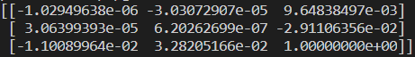
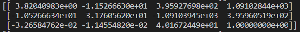
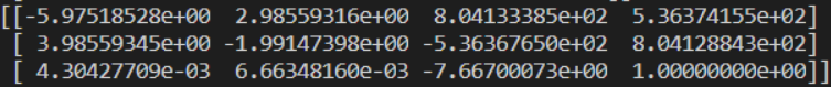
图2的相机矩阵为:
经过处理后的特征匹配为:

图1和图3的匹配结果为:

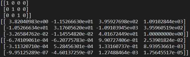
三张图的相机矩阵为:
2. 室外
这组拍摄了三张照片,按照从远到近的顺序分别为图1,2,3
图1和图2的sift特征匹配结果为:

得到的基础矩阵为:
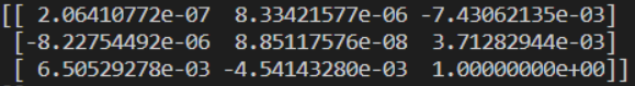
图2的照相机矩阵为:
经过处理后的特征匹配为:

图1和图3的匹配结果:

三张图的相机矩阵为:

结果分析:
可能由于拍摄问题,两组实验结果都不是很理想,特征匹配均出现了一些偏差。
整体实验过程中发现室内取材远远难于室外,室外使用一组图片就通过了运行,而室内至少采集了七八组,但运行到一半大多数都出现了下面这个错误:

个人感觉是因为室内拍摄时,从图像很难反映出明显的景深差距(当然也可能是我个人拍摄问题…),室外相对拍摄景深差距较大。当然还有光照一些因素导致没有特征匹配点。
匹配结果而言对于环境更加复杂的室内,特征匹配点更少,但是更精确,而室外的特征虽然都远远多于室内,但是存在一些相似的特征点而导致匹配错误。


 3062
3062


 被折叠的 条评论
为什么被折叠?
被折叠的 条评论
为什么被折叠?
 到【灌水乐园】发言


