【深度学习】ResNet网络讲解

大龙唉

已于 2023-11-03 03:56:19 修改

阅读量1.4w

点赞数 41

文章标签：深度学习人工智能

于 2023-11-03 03:29:23 首次发布

本文链接：https://blog.csdn.net/weixin_44001371/article/details/134192776

版权

ResNet中两种不同的ResNet block

网络结构

六、ResNet-layers模型完整代码

1. BasicBlock

2. BottleNeck

3. ResNet

4. 搭建ResNet-34、ResNet-50模型

【附录：ResNet_layer模型代码】

参考链接

【DL系列】ResNet网络结构详解、完整代码实现

你必须要知道CNN模型：ResNet

6.1 ResNet网络结构，BN以及迁移学习详解

【深度学习】ResNet网络详解

ResNet详解

一、什么是ResNet？

ResNet网络是在2015年由微软实验室中的何凯明等几位大神提出，论文地址是《Deep Residual Learning for Image Recognition》；是在CVPR 2016发表的一种影响深远的网络模型，由何凯明大神团队提出来，在ImageNet的分类比赛上将网络深度直接提高到了152层，前一年夺冠的VGG只有19层。斩获当年ImageNet竞赛中分类任务第一名，目标检测第一名。获得COCO数据集中目标检测第一名，图像分割第一名，可以说ResNet的出现对深度神经网络来说具有重大的历史意义。

Resnet在cnn图像方面有着非常突出的表现，它利用 shortcut 短路连接，解决了深度网络中模型退化的问题。相比普通网络每两层/三层之间增加了短路机制，通过残差学习使深层的网络发挥出作用。

二、网络中的亮点

1.超深的网络结构（超过1000层）。
2.提出residual（残差结构）模块。
3.使用Batch Normalization加速训练（丢弃dropout）。

三、为什么采用residual?

在ResNet提出之前，所有的神经网络都是通过卷积层和池化层的叠加组成的。
人们认为卷积层和池化层的层数越多，获取到的图片特征信息越全，学习效果也就越好。但是在实际的试验中发现，随着卷积层和池化层的叠加，不但没有出现学习效果越来越好的情况，反而出现

两种问题：

1.梯度消失和梯度爆炸

梯度消失：若每一层的误差梯度小于1，反向传播时，网络越深，梯度越趋近于0
梯度爆炸：若每一层的误差梯度大于1，反向传播时，网络越深，梯度越来越大

2.退化问题

随着层数的增加，预测效果反而越来越差。如下图所示

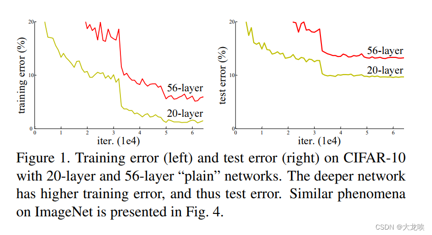
从图中可以看出错误率在20层时候是最低的，添加到了56层反而更高了。可能会有小伙伴说是不是过拟合了（模型在训练数据上表现很好，但在未见过的新数据上表现较差）？其实可以看出来，如果是你过拟合的话，左侧的训练接在56层时候的错误率依然上升，所以并不是过拟合产生的该情况，是由于神经网络在反向传播过程中通过链式法则不断地反向传播更新梯度，而当网络层数加深时，梯度在传播过程中会逐渐消失也就说我们所说的梯度弥散。这将导致无法对前面网络层的权重进行有效的调整，网络层数越深，训练误差越高，导致训练和测试效果变差，这一现象称为退化。那么，理论上本应该层次更深、效果更好的神经网络，实验结果反而不好，该怎么解决这个问题呢？很多学者都为此感到头疼，幸好RestNet姗姗赶来。

解决方法

为了解决梯度消失或梯度爆炸问题，ResNet论文提出通过数据的预处理以及在网络中使用 BN（Batch Normalization）层来解决。
为了解决深层网络中的退化问题，可以人为地让神经网络某些层跳过下一层神经元的连接，隔层相连，弱化每层之间的强联系。这种神经网络被称为残差网络 (ResNets)。ResNet论文提出了 residual结构（残差结构）来减轻退化问题，下图是使用residual结构的卷积网络，可以看到随着网络的不断加深，效果并没有变差，而是变的更好了。（虚线是train error，实线是test error）

四、残差学习

残差即观测值 $H(x)$ 与估计值 $x$ 之间的差。

深度网络的退化问题至少说明深度网络不容易训练。但是我们考虑这样一个事实：现在你有一个浅层网络，你想通过向上堆积新层来建立深层网络，一个极端情况是这些增加的层什么也不学习，仅仅复制浅层网络的特征，即这样新层是恒等映射（Identity mapping）。在这种情况下，深层网络应该至少和浅层网络性能一样，那么退化问题就得到了解决。

传统的CNN网络如左图所示，这是一个普通的、两层的卷积+激活。经过两层卷积+一个激活，我们假定它输出为H(x)。与传统的网络结构相比，ResNet增加了短路连接(shortcut connection)或称为跳跃连接(skip connection) ，如右图所示：

这其实就是残差块的关键点所在，它添加了一个短路连接到第二层激活函数之前。那么激活函数的输入就由原来的输出H(x)=F(x)变为了H(x)=F(x)+x。在RestNet中，这种输出=输入的操作成为恒等映射（Identity mapping）。通过这种操作，使得网络在最差的情况下也能获得和输入一样的输出，即增加的层什么也不学习，仅仅复制输入的特征，至少使得网络不会出现退化的问题。

从数学角度分析一下：

$\begin{array}{l} \mathrm{y}_{\mathrm{l}}=\mathrm{h}\left(\mathrm{x}_{\mathrm{l}}\right)+\mathrm{F}\left(\mathrm{x}_{\mathrm{l}}, \mathrm{W}_{\mathrm{l}}\right) \\ \mathrm{x}_{\mathrm{l}+1}=\mathrm{f}\left(\mathrm{y}_{\mathrm{l}}\right) \end{array}$

其中 $\mathrm{x}_{\mathrm{l}}$ 和 $\mathrm{x}_{\mathrm{l}+1}$ 分别表示的是第 $l$ 个残差单元的输入和输出，注意每个残差单元一般包含多层结构。 $F$ 是残差函数，表示学习到的残差，而 $h(x_l)=x_l$ 表示恒等映射， $f$ 是ReLU激活函数。基于上式，我们求得从浅层 $l$ 到深层 $L$ 的学习特征为：

$x_{L}=x_{l}+\sum_{i=l}^{L-1} F\left(x_{i}, W_{i}\right)$

五、ResNet的网络结构

ResNet中两种不同的ResNet block

ResNet block有两种，一种左侧两层的BasicBlock结构，一种是右侧三层的bottleneck结构，即将两个 $3\times 3$ 的卷积层替换为 $1\times 1+3\times 3+1\times 1$ ，它通过 $1\times 1$ conv来巧妙地缩减或扩张feature map维度，从而使得我们的 $3\times 3$ conv的filters数目不受上一层输入的影响，它的输出也不会影响到下一层。中间 $3\times 3$ 的卷积层首先在一个降维 $1\times 1$ 卷积层下减少了计算，然后在另一个 $1\times 1$ 的卷积层下做了还原。既保持了模型精度又减少了网络参数和计算量，节省了计算时间。

注意：搭建深层次网络时，采用三层的残差结构（bottleneck）。

先降后升为了主分支上输出的特征矩阵和捷径分支上输出的特征矩阵形状相同，以便进行加法操作。

注：CNN参数个数 = 卷积核尺寸×卷积核深度 × 卷积核组数 = 卷积核尺寸 × 输入特征矩阵深度 × 输出特征矩阵深度

注意：
对于短路连接，如果残差映射 $F(x)$ 的维度与跳跃连接x的维度不同，那咱们是没有办法对它们两个进行相加操作的，必须对 $x$ 进行升维操作，让他俩的维度相同时才能计算：

zero-padding全0填充增加维度：
- 此时一般要先做一个downsamp，可以采用stride=2的pooling，这样不会增加参数
采用新的映射（projection shortcut）：
- 一般采用1x1的卷积，这样会增加参数，也会增加计算量。

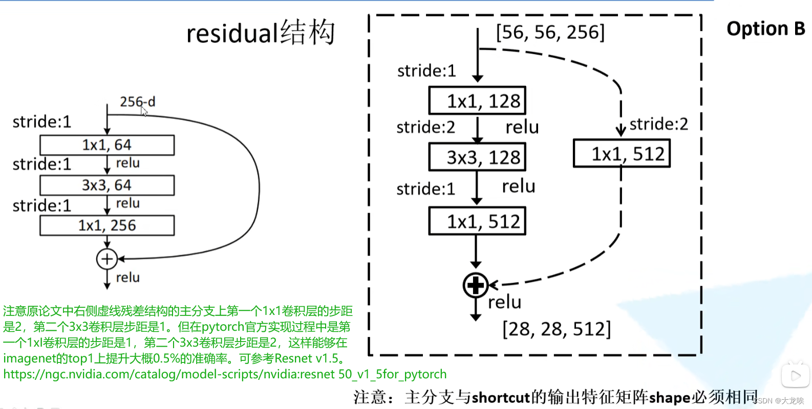
在resnet结构中，主分支与shortcut的输出特征矩阵shape必须相同，因此，如下图右侧所示虚线残差结构，在捷径分支上通过1x1的卷积核进行降维处理，并通过设置步长为2来改变分辨率，最终实现维度的匹配：

网络结构

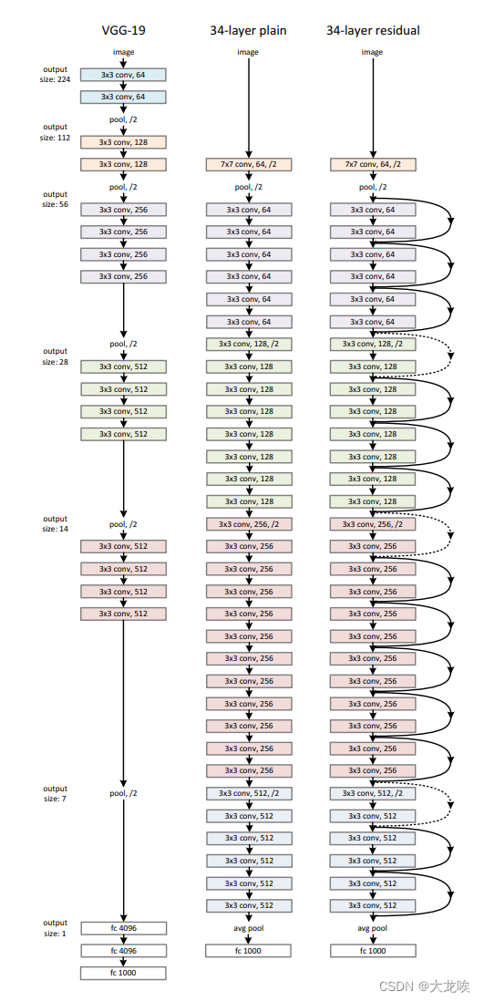
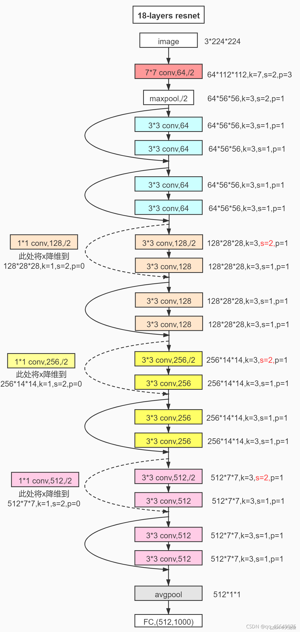
ResNet网络是参考了VGG19网络，在其基础上进行了修改，并通过短路机制加入了残差单元，如下图所示。变化主要体现在ResNet直接使用stride=2的卷积做下采样，并且用global average pool层替换了全连接层。ResNet的一个重要设计原则是：当feature map大小降低一半时，feature map的数量增加一倍，这保持了网络层的复杂度。从下图中可以看到，ResNet相比普通网络每两层间增加了短路机制，这就形成了残差学习，其中虚线表示feature map数量发生了改变，即使用了虚线残差结构，通过1*1卷积来改变维度。下图展示的34-layer的ResNet，还可以构建更深的网络如表1所示。从表中可以看到，对于18-layer和34-layer的ResNet，其进行的两层间的残差学习，当网络更深时，其进行的是三层间的残差学习，三层卷积核分别是1x1，3x3和1x1。

ResNet的网络结构图如图所示：

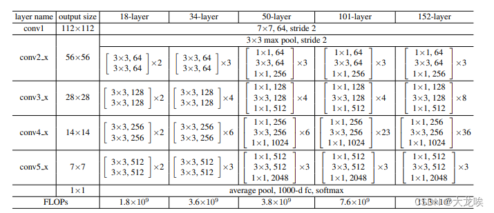
这是ResNet不同层数的网络结构图。

可以看到，结构大差不差。不论是18层、34层、50层、还是101层、152层。

上来都是一个7x7的卷积层，然后是一个3x3的最大池化下采样。

然后就是按照图中的conv2_x、conv3_x、conv4_x、conv5_x中的残差结构。

最后再跟一个平均池化下采样，和全连接层，sofmax输出。

首先，ResNet使用ImagesNet数据集，采用的默认输入尺寸是(224, 224, 3)，RGB图像，三通道

按照表中，我们可以看到，图片输入之后，首先是一个7x7,64,stride 2

也就是一个卷积层，卷积核大小为7x7，输出通道为64（也就是卷积核个数），stride=2。

没说padding，我们需要自己算一下，表里写了这一层的输出是112x112

补充一点知识：

假设输入图片为 W x W 卷积核大小为F x F，步长stride=S，padding=P（填充的像素数）
则输出图像的大小 W2 =（W - F +2P）/S +1

可以注意到这个公式中有除法，一般我们做卷积时除不尽的时候都向下取整

可以参考pytorch官方文档：https://pytorch.org/docs/stable/generated/torch.nn.Conv2d.html#torch.nn.Conv2d

但是我们做池化的时候，也可以采用向上取整

参看pytorch官方文档：https://pytorch.org/docs/stable/generated/torch.nn.MaxPool2d.html#torch.nn.MaxPool2d

有一个参数ceil_mode，默认是floor是向下取整，可以设置为True，向上取整
ceil_mode – when True, will use ceil instead of floor to compute the output shape
有的时候池化会选择向上取整（最大池化和平均池化有时取整方式不同）

那就是说 112 = （224 - 7 + 2P）/ 2 + 1

化简后就是 111 = （217 + 2P）/2 = 108.5+P

所以P=3 所以Padding是3

所以我们输入图片进来，第一层

in_channel=3,out_channel=64,kernel_size=7,stride=2,padding=3

没有偏置bias。经过这一层我们会得到大小为112x112的尺寸，通道数为64

然后经过一个3x3的最大池化下采样，stride=2

$W_{out}=(W_{in}-F+2P)/S+1$

池化层也采用向下取整。所以 56=(112 - 3 + 2P)/2 +1 计算出来P=1

所以第二层池化层是

in_channel=3,out_channel=64,kernel_size=7,stride=2,padding=3

经过池化层，我们会得到一个56x56，64通道的输出，紧接着就是conv2_xconv2_x、conv3_x、conv4_x、conv5_x中对应的一系列残差结构，Resnet-18网络中具体的卷积和数和输入输出特征图大小如下图所示：

六、ResNet-layers模型完整代码

【注】： 此模型代码与Pytorch官方源码结构逻辑基本一致。具体细节问题，代码中注释已给出解释和说明。

1. BasicBlock

import torch
import torch.nn as nn


class BasicBlock(nn.Module):
    """搭建BasicBlock模块"""
    expansion = 1

    def __init__(self, in_channel, out_channel, stride=1, downsample=None):
        super(BasicBlock, self).__init__()

        # 使用BN层是不需要使用bias的，bias最后会抵消掉
        self.conv1 = nn.Conv2d(in_channel, out_channel, kernel_size=3, padding=1, stride=stride, bias=False)
        self.bn1 = nn.BatchNorm2d(out_channel)    # BN层, BN层放在conv层和relu层中间使用
        self.conv2 = nn.Conv2d(out_channel, out_channel, kernel_size=3, padding=1, bias=False)
        self.bn2 = nn.BatchNorm2d(out_channel)

        self.downsample = downsample
        self.relu = nn.ReLU(inplace=True)

    # 前向传播
    def forward(self, X):
        identity = X
        Y = self.relu(self.bn1(self.conv1(X)))
        Y = self.bn2(self.conv2(Y))

        if self.downsample is not None:    # 保证原始输入X的size与主分支卷积后的输出size叠加时维度相同
            identity = self.downsample(X)

        return self.relu(Y + identity)

2. BottleNeck

class BottleNeck(nn.Module):
    """搭建BottleNeck模块"""
    # BottleNeck模块最终输出out_channel是Residual模块输入in_channel的size的4倍(Residual模块输入为64)，shortcut分支in_channel
    # 为Residual的输入64，因此需要在shortcut分支上将Residual模块的in_channel扩张4倍，使之与原始输入图片X的size一致
    expansion = 4

    def __init__(self, in_channel, out_channel, stride=1, downsample=None):
        super(BottleNeck, self).__init__()

        # 默认原始输入为256，经过7x7层和3x3层之后BottleNeck的输入降至64
        self.conv1 = nn.Conv2d(in_channel, out_channel, kernel_size=1, bias=False)
        self.bn1 = nn.BatchNorm2d(out_channel)    # BN层, BN层放在conv层和relu层中间使用
        self.conv2 = nn.Conv2d(out_channel, out_channel, kernel_size=3, stride=stride, padding=1, bias=False)
        self.bn2 = nn.BatchNorm2d(out_channel)
        self.conv3 = nn.Conv2d(out_channel, out_channel * self.expansion, kernel_size=1, bias=False)
        self.bn3 = nn.BatchNorm2d(out_channel * self.expansion)  # Residual中第三层out_channel扩张到in_channel的4倍

        self.downsample = downsample
        self.relu = nn.ReLU(inplace=True)

    # 前向传播
    def forward(self, X):
        identity = X

        Y = self.relu(self.bn1(self.conv1(X)))
        Y = self.relu(self.bn2(self.conv2(Y)))
        Y = self.bn3(self.conv3(Y))

        if self.downsample is not None:    # 保证原始输入X的size与主分支卷积后的输出size叠加时维度相同
            identity = self.downsample(X)

        return self.relu(Y + identity)

3. ResNet

class ResNet(nn.Module):
    """搭建ResNet-layer通用框架"""
    # num_classes是训练集的分类个数，include_top是在ResNet的基础上搭建更加复杂的网络时用到，此处用不到
    def __init__(self, residual, num_residuals, num_classes=1000, include_top=True):
        super(ResNet, self).__init__()

        self.out_channel = 64    # 输出通道数(即卷积核个数)，会生成与设定的输出通道数相同的卷积核个数
        self.include_top = include_top

        self.conv1 = nn.Conv2d(3, self.out_channel, kernel_size=7, stride=2, padding=3,
                               bias=False)    # 3表示输入特征图像的RGB通道数为3，即图片数据的输入通道为3
        self.bn1 = nn.BatchNorm2d(self.out_channel)
        self.relu = nn.ReLU(inplace=True)
        self.maxpool = nn.MaxPool2d(kernel_size=3, stride=2, padding=1)
        self.conv2 = self.residual_block(residual, 64, num_residuals[0])
        self.conv3 = self.residual_block(residual, 128, num_residuals[1], stride=2)
        self.conv4 = self.residual_block(residual, 256, num_residuals[2], stride=2)
        self.conv5 = self.residual_block(residual, 512, num_residuals[3], stride=2)
        if self.include_top:
            self.avgpool = nn.AdaptiveAvgPool2d((1, 1))    # output_size = (1, 1)
            self.fc = nn.Linear(512 * residual.expansion, num_classes)

        # 对conv层进行初始化操作
        for m in self.modules():
            if isinstance(m, nn.Conv2d):
                nn.init.kaiming_normal_(m.weight, mode='fan_out', nonlinearity='relu')
            elif isinstance(m, (nn.BatchNorm2d, nn.GroupNorm)):
                nn.init.constant_(m.weight, 1)
                nn.init.constant_(m.bias, 0)

    def residual_block(self, residual, channel, num_residuals, stride=1):
        downsample = None

        # 用在每个conv_x组块的第一层的shortcut分支上，此时上个conv_x输出out_channel与本conv_x所要求的输入in_channel通道数不同，
        # 所以用downsample调整进行升维，使输出out_channel调整到本conv_x后续处理所要求的维度。
        # 同时stride=2进行下采样减小尺寸size，(注：conv2时没有进行下采样，conv3-5进行下采样，size=56、28、14、7)。
        if stride != 1 or self.out_channel != channel * residual.expansion:
            downsample = nn.Sequential(
                nn.Conv2d(self.out_channel, channel * residual.expansion, kernel_size=1, stride=stride, bias=False),
                nn.BatchNorm2d(channel * residual.expansion))

        block = []    # block列表保存某个conv_x组块里for循环生成的所有层
        # 添加每一个conv_x组块里的第一层，第一层决定此组块是否需要下采样(后续层不需要)
        block.append(residual(self.out_channel, channel, downsample=downsample, stride=stride))
        self.out_channel = channel * residual.expansion    # 输出通道out_channel扩张

        for _ in range(1, num_residuals):
            block.append(residual(self.out_channel, channel))

        # 非关键字参数的特征是一个星号*加上参数名，比如*number，定义后，number可以接收任意数量的参数，并将它们储存在一个tuple中
        return nn.Sequential(*block)

    # 前向传播
    def forward(self, X):
        Y = self.relu(self.bn1(self.conv1(X)))
        Y = self.maxpool(Y)
        Y = self.conv5(self.conv4(self.conv3(self.conv2(Y))))

        if self.include_top:
            Y = self.avgpool(Y)
            Y = torch.flatten(Y, 1)
            Y = self.fc(Y)

        return Y

4. 搭建ResNet-34、ResNet-50模型

# 构建ResNet-34模型
def resnet34(num_classes=1000, include_top=True):
    return ResNet(BasicBlock, [3, 4, 6, 3], num_classes=num_classes, include_top=include_top)


# 构建ResNet-50模型
def resnet50(num_classes=1000, include_top=True):
    return ResNet(BottleNeck, [3, 4, 6, 3], num_classes=num_classes, include_top=include_top)


# 模型网络结构可视化
net = resnet34()

5. 网络结构可视化

# 1. 使用torchsummary中的summary查看模型的输入输出形状、顺序结构，网络参数量，网络模型大小等信息
from torchsummary import summary

device = torch.device("cuda" if torch.cuda.is_available() else "cpu")
model = net.to(device)
summary(model, (3, 224, 224))    # 3是RGB通道数，即表示输入224 * 224的3通道的数据


# 2. 使用torchviz中的make_dot生成模型的网络结构，pdf图包括计算路径、网络各层的权重、偏移量
from torchviz import make_dot

X = torch.rand(size=(1, 3, 224, 224))    # 3是RGB通道数，即表示输入224 * 224的3通道的数据
Y = net(X)
vise = make_dot(Y, params=dict(net.named_parameters()))
vise.view()

6. 查看Pytorch官方源码

# Pytorch官方ResNet模型
# 导入resnet包，(ctrl + 左键)点击resnet34，即可查看resnet-layer模型源码
from torchvision.models import resnet34

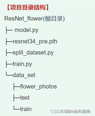
7. split_dataset.py

文件： split_dataset.py

功能：数据集划分脚本。将原始数据集 flower_photos 划分为 train 和 test 两个数据集，并更改图片size=224x224。

数据集下载地址：http://download.tensorflow.org/example_images/flower_photos.tgz

数据集保存路径：根目录 \ data_set \ flower_photos

"""
# 数据集划分脚本
#
"""

import os
import glob
import random
from PIL import Image


if __name__ == '__main__':
    split_rate = 0.1    # 训练集和验证集划分比率
    resize_image = 224    # 图片缩放后统一大小
    file_path = '.\\data_set\\flower_photos'    # 获取原始数据集路径

    # 找到文件中所有文件夹的目录，即类文件夹名
    dirs = glob.glob(os.path.join(file_path, '*'))
    dirs = [d for d in dirs if os.path.isdir(d)]

    print("Totally {} classes: {}".format(len(dirs), dirs))    # 打印花类文件夹名称

    for path in dirs:
        # 对每个类别进行单独处理
        path = path.split('\\')[-1]  # -1表示以分隔符/保留后面的一段字符

        # 在根目录中创建两个文件夹，train/test
        os.makedirs("data_set\\train\\{}".format(path), exist_ok=True)
        os.makedirs("data_set\\test\\{}".format(path), exist_ok=True)

        # 读取原始数据集中path类中对应类型的图片，并添加到files中
        files = glob.glob(os.path.join(file_path, path, '*jpg'))
        files += glob.glob(os.path.join(file_path, path, '*jpeg'))
        files += glob.glob(os.path.join(file_path, path, '*png'))

        random.shuffle(files)    # 打乱图片顺序
        split_boundary = int(len(files) * split_rate)  # 训练集和测试集的划分边界

        for i, file in enumerate(files):
            img = Image.open(file).convert('RGB')

            # 更改原始图片尺寸
            old_size = img.size  # (wight, height)
            ratio = float(resize_image) / max(old_size)  # 通过最长的size计算原始图片缩放比率
            # 把原始图片最长的size缩放到resize_pic，短的边等比率缩放，等比例缩放不会改变图片的原始长宽比
            new_size = tuple([int(x * ratio) for x in old_size])

            im = img.resize(new_size, Image.ANTIALIAS)  # 更改原始图片的尺寸，并设置图片高质量，保存成新图片im
            new_im = Image.new("RGB", (resize_image, resize_image))  # 创建一个resize_pic尺寸的黑色背景
            # 把新图片im贴到黑色背景上，并通过'地板除//'设置居中放置
            new_im.paste(im, ((resize_image - new_size[0]) // 2, (resize_image - new_size[1]) // 2))

            # 先划分0.1_rate的测试集，剩下的再划分为0.9_ate的训练集，同时直接更改图片后缀为.jpg
            assert new_im.mode == "RGB"
            if i < split_boundary:
                new_im.save(os.path.join("data_set\\test\\{}".format(path),
                                         file.split('\\')[-1].split('.')[0] + '.jpg'))
            else:
                new_im.save(os.path.join("data_set\\train\\{}".format(path),
                                         file.split('\\')[-1].split('.')[0] + '.jpg'))

    # 统计划分好的训练集和测试集中.jpg图片的数量
    train_files = glob.glob(os.path.join('data_set', 'train', '*', '*.jpg'))
    test_files = glob.glob(os.path.join('data_set', 'test', '*', '*.jpg'))

    print("Totally {} files for train".format(len(train_files)))
    print("Totally {} files for test".format(len(test_files)))

8. train.py

文件： train.py

功能：训练模型和验证训练好的模型精度。

ResNet-34 预训练权重文件下载地址： https://download.pytorch.org/models/resnet34-b627a593.pth

【注】：其它ResNet-layer预训练权重下载地址：

model_urls = {
    'resnet18': 'https://download.pytorch.org/models/resnet18-f37072fd.pth',
    'resnet34': 'https://download.pytorch.org/models/resnet34-b627a593.pth',
    'resnet50': 'https://download.pytorch.org/models/resnet50-0676ba61.pth',
    'resnet101': 'https://download.pytorch.org/models/resnet101-63fe2227.pth',
    'resnet152': 'https://download.pytorch.org/models/resnet152-394f9c45.pth',
    'resnext50_32x4d': 'https://download.pytorch.org/models/resnext50_32x4d-7cdf4587.pth',
    'resnext101_32x8d': 'https://download.pytorch.org/models/resnext101_32x8d-8ba56ff5.pth',
    'wide_resnet50_2': 'https://download.pytorch.org/models/wide_resnet50_2-95faca4d.pth',
    'wide_resnet101_2': 'https://download.pytorch.org/models/wide_resnet101_2-32ee1156.pth',
}

"""
# 训练脚本
#
"""

import os
import sys
import json
import time

import torch
import torch.nn as nn
import torch.optim as optim
import torch.utils.data as Data
from torchvision import transforms, datasets
from tqdm import tqdm

from model import resnet34


def train_model():
    device = torch.device("cuda:0" if torch.cuda.is_available() else "cpu")
    print("Using {} device.".format(device))

    # 数据预处理。transforms提供一系列数据预处理方法
    data_transform = {
        "train": transforms.Compose([transforms.RandomResizedCrop(224),    # 随机裁剪
                                     transforms.RandomHorizontalFlip(),    # 水平方向随机反转
                                     transforms.ToTensor(),
                                     transforms.Normalize([0.485, 0.456, 0.406], [0.229, 0.224, 0.225])]),    # 标准化
        "val": transforms.Compose([transforms.Resize(256),    # 图像缩放
                                   transforms.CenterCrop(224),    # 中心裁剪
                                   transforms.ToTensor(),
                                   transforms.Normalize([0.485, 0.456, 0.406], [0.229, 0.224, 0.225])])}

    # 获取数据集根目录(即当前代码文件夹路径)
    data_root = os.path.abspath(os.path.join(os.getcwd(), ".\\"))
    # 获取flower图片数据集路径
    image_path = os.path.join(data_root, "data_set")
    assert os.path.exists(image_path), "{} path does not exist.".format(image_path)

    # ImageFolder是一个通用的数据加载器，它要求我们以root/class/xxx.png格式来组织数据集的训练、验证或者测试图片。
    train_dataset = datasets.ImageFolder(root=os.path.join(image_path, "train"), transform=data_transform["train"])
    train_num = len(train_dataset)
    val_dataset = datasets.ImageFolder(root=os.path.join(image_path, "test"), transform=data_transform["val"])
    val_num = len(val_dataset)

    # {'daisy':0, 'dandelion':1, 'roses':2, 'sunflower':3, 'tulips':4}
    flower_list = train_dataset.class_to_idx
    class_dict = dict((val, key) for key, val in flower_list.items())    # 将字典中键值对翻转。此处翻转为 {'0':daisy,...}

    # 将class_dict编码成json格式文件
    json_str = json.dumps(class_dict, indent=4)
    with open('class_indices.json', 'w') as json_file:
        json_file.write(json_str)

    batch_size = 4    # 设置批大小。batch_size太大会报错OSError: [WinError 1455] 页面文件太小，无法完成操作。
    num_workers = min([os.cpu_count(), batch_size if batch_size > 1 else 0, 8])  # number of workers
    print("Using batch_size={} dataloader workers every process.".format(num_workers))

    # 加载训练集和测试集
    train_loader = Data.DataLoader(train_dataset, batch_size=batch_size,
                                   num_workers=num_workers, shuffle=True)
    val_loader = Data.DataLoader(val_dataset, batch_size=batch_size,
                                 num_workers=num_workers, shuffle=True)
    print("Using {} train_images for training, {} test_images for validation.".format(train_num, val_num))
    print()

    # 加载预训练权重
    # download url: https://download.pytorch.org/models/resnet34-b627a593.pth
    net = resnet34()
    model_weight_path = ".\\resnet34_pre.pth"    # 预训练权重
    assert os.path.exists(model_weight_path), "file {} does not exist.".format(model_weight_path)
    # torch.load_state_dict()函数就是用于将预训练的参数权重加载到新的模型之中
    net.load_state_dict(torch.load(model_weight_path, map_location='cpu'), strict=False)

    # 改变in_channel符合fc层的要求，调整output为数据集类别5
    in_channel = net.fc.in_features
    net.fc = nn.Linear(in_channel, 5)
    net.to(device)

    # 损失函数
    loss_function = nn.CrossEntropyLoss()

    # 优化器
    params = [p for p in net.parameters() if p.requires_grad]
    optimizer = optim.Adam(params, lr=0.0001)

    epochs = 10    # 训练迭代次数
    best_acc = 0.0
    save_path = '.\\resNet34.pth'    # 当前模型训练好后的权重参数文件保存路径
    batch_num = len(train_loader)    # 一个batch中数据的数量
    total_time = 0    # 统计训练过程总时间

    for epoch in range(epochs):
        # 开始迭代训练和测试
        start_time = time.perf_counter()  # 计算训练一个epoch的时间

        # train
        net.train()
        train_loss = 0.0
        train_bar = tqdm(train_loader, file=sys.stdout)    # tqdm是Python进度条库，可以在Python长循环中添加一个进度条提示信息。

        for step, data in enumerate(train_bar):
            train_images, train_labels = data
            train_images = train_images.to(device)
            train_labels = train_labels.to(device)

            optimizer.zero_grad()    # 梯度置零。清空之前的梯度信息
            outputs = net(train_images)    # 前向传播
            loss = loss_function(outputs, train_labels)    # 计算损失
            loss.backward()    # 反向传播
            optimizer.step()    # 参数更新
            train_loss += loss.item()    # 将计算的loss累加到train_loss中

            # desc：str类型，作为进度条说明，在进度条右边
            train_bar.desc = "train epoch[{}/{}] loss:{:.3f}.".format(epoch+1, epochs, loss)

        # validate
        net.eval()
        val_acc = 0.0
        val_bar = tqdm(val_loader, file=sys.stdout)

        with torch.no_grad():
            for val_data in val_bar:
                val_images, val_labels = val_data
                val_images = val_images.to(device)
                val_labels = val_labels.to(device)

                val_y = net(val_images)    # 前向传播
                predict_y = torch.max(val_y, dim=1)[1]    # 在维度为1上找到预测Y的最大值，第0个维度是batch
                # 计算测试集精度。predict_y与val_labels进行比较(true=1, False=0)的一个batch求和，所有batch的累加精度值
                val_acc += torch.eq(predict_y, val_labels).sum().item()

                val_bar.desc = "valid epoch[{}/{}].".format(epoch+1, epochs)

        # 打印epoch数据结果
        val_accurate = val_acc / val_num
        print("[epoch {:.0f}] train_loss: {:.3f}  val_accuracy: {:.3f}"
              .format(epoch+1, train_loss/batch_num, val_accurate))

        epoch_time = time.perf_counter() - start_time    # 计算训练一个epoch的时间
        print("epoch_time: {}".format(epoch_time))
        total_time += epoch_time    # 统计训练过程总时间
        print()

        # 调整测试集最优精度
        if val_accurate > best_acc:
            best_acc = val_accurate
            # model.state_dict()保存学习到的参数
            torch.save(net.state_dict(), save_path)    # 保存当前最高的准确度

    # 将训练过程总时间转换为h:m:s格式打印
    m, s = divmod(total_time, 60)
    h, m = divmod(m, 60)
    print("Total_time: {:.0f}:{:.0f}:{:.0f}".format(h, m, s))

    print('Finished Training!')


if __name__ == '__main__':
    train_model()

【附录：ResNet_layer模型代码】

文件： model.py

"""
# 搭建resnet-layer模型
#
"""
import torch
import torch.nn as nn


class BasicBlock(nn.Module):
    """搭建BasicBlock模块"""
    expansion = 1

    def __init__(self, in_channel, out_channel, stride=1, downsample=None):
        super(BasicBlock, self).__init__()

        # 使用BN层是不需要使用bias的，bias最后会抵消掉
        self.conv1 = nn.Conv2d(in_channel, out_channel, kernel_size=3, padding=1, stride=stride, bias=False)
        self.bn1 = nn.BatchNorm2d(out_channel)    # BN层, BN层放在conv层和relu层中间使用
        self.conv2 = nn.Conv2d(out_channel, out_channel, kernel_size=3, padding=1, bias=False)
        self.bn2 = nn.BatchNorm2d(out_channel)

        self.downsample = downsample
        self.relu = nn.ReLU(inplace=True)

    # 前向传播
    def forward(self, X):
        identity = X
        Y = self.relu(self.bn1(self.conv1(X)))
        Y = self.bn2(self.conv2(Y))

        if self.downsample is not None:    # 保证原始输入X的size与主分支卷积后的输出size叠加时维度相同
            identity = self.downsample(X)

        return self.relu(Y + identity)


class BottleNeck(nn.Module):
    """搭建BottleNeck模块"""
    # BottleNeck模块最终输出out_channel是Residual模块输入in_channel的size的4倍(Residual模块输入为64)，shortcut分支in_channel
    # 为Residual的输入64，因此需要在shortcut分支上将Residual模块的in_channel扩张4倍，使之与原始输入图片X的size一致
    expansion = 4

    def __init__(self, in_channel, out_channel, stride=1, downsample=None):
        super(BottleNeck, self).__init__()
        # 默认原始输入为224，经过7x7层和3x3层之后BottleNeck的输入降至64
        self.conv1 = nn.Conv2d(in_channel, out_channel, kernel_size=1, bias=False)
        self.bn1 = nn.BatchNorm2d(out_channel)    # BN层, BN层放在conv层和relu层中间使用
        self.conv2 = nn.Conv2d(out_channel, out_channel, kernel_size=3, stride=stride, padding=1, bias=False)
        self.bn2 = nn.BatchNorm2d(out_channel)
        self.conv3 = nn.Conv2d(out_channel, out_channel * self.expansion, kernel_size=1, bias=False)
        self.bn3 = nn.BatchNorm2d(out_channel * self.expansion)  # Residual中第三层out_channel扩张到in_channel的4倍

        self.downsample = downsample
        self.relu = nn.ReLU(inplace=True)

    # 前向传播
    def forward(self, X):
        identity = X

        Y = self.relu(self.bn1(self.conv1(X)))
        Y = self.relu(self.bn2(self.conv2(Y)))
        Y = self.bn3(self.conv3(Y))

        if self.downsample is not None:    # 保证原始输入X的size与主分支卷积后的输出size叠加时维度相同
            identity = self.downsample(X)

        return self.relu(Y + identity)


class ResNet(nn.Module):
    """搭建ResNet-layer通用框架"""
    # num_classes是训练集的分类个数，include_top是在ResNet的基础上搭建更加复杂的网络时用到，此处用不到
    def __init__(self, residual, num_residuals, num_classes=1000, include_top=True):
        super(ResNet, self).__init__()

        self.out_channel = 64    # 输出通道数(即卷积核个数)，会生成与设定的输出通道数相同的卷积核个数
        self.include_top = include_top

        self.conv1 = nn.Conv2d(3, self.out_channel, kernel_size=7, stride=2, padding=3,
                               bias=False)    # 3表示输入特征图像的RGB通道数为3，即图片数据的输入通道为3
        self.bn1 = nn.BatchNorm2d(self.out_channel)
        self.relu = nn.ReLU(inplace=True)
        self.maxpool = nn.MaxPool2d(kernel_size=3, stride=2, padding=1)
        self.conv2 = self.residual_block(residual, 64, num_residuals[0])
        self.conv3 = self.residual_block(residual, 128, num_residuals[1], stride=2)
        self.conv4 = self.residual_block(residual, 256, num_residuals[2], stride=2)
        self.conv5 = self.residual_block(residual, 512, num_residuals[3], stride=2)
        if self.include_top:
            self.avgpool = nn.AdaptiveAvgPool2d((1, 1))    # output_size = (1, 1)
            self.fc = nn.Linear(512 * residual.expansion, num_classes)

        # 对conv层进行初始化操作
        for m in self.modules():
            if isinstance(m, nn.Conv2d):
                nn.init.kaiming_normal_(m.weight, mode='fan_out', nonlinearity='relu')
            elif isinstance(m, (nn.BatchNorm2d, nn.GroupNorm)):
                nn.init.constant_(m.weight, 1)
                nn.init.constant_(m.bias, 0)

    def residual_block(self, residual, channel, num_residuals, stride=1):
        downsample = None

        # 用在每个conv_x组块的第一层的shortcut分支上，此时上个conv_x输出out_channel与本conv_x所要求的输入in_channel通道数不同，
        # 所以用downsample调整进行升维，使输出out_channel调整到本conv_x后续处理所要求的维度。
        # 同时stride=2进行下采样减小尺寸size，(注：conv2时没有进行下采样，conv3-5进行下采样，size=56、28、14、7)。
        if stride != 1 or self.out_channel != channel * residual.expansion:
            downsample = nn.Sequential(
                nn.Conv2d(self.out_channel, channel * residual.expansion, kernel_size=1, stride=stride, bias=False),
                nn.BatchNorm2d(channel * residual.expansion))

        block = []    # block列表保存某个conv_x组块里for循环生成的所有层
        # 添加每一个conv_x组块里的第一层，第一层决定此组块是否需要下采样(后续层不需要)
        block.append(residual(self.out_channel, channel, downsample=downsample, stride=stride))
        self.out_channel = channel * residual.expansion    # 输出通道out_channel扩张

        for _ in range(1, num_residuals):
            block.append(residual(self.out_channel, channel))

        # 非关键字参数的特征是一个星号*加上参数名，比如*number，定义后，number可以接收任意数量的参数，并将它们储存在一个tuple中
        return nn.Sequential(*block)

    # 前向传播
    def forward(self, X):
        Y = self.relu(self.bn1(self.conv1(X)))
        Y = self.maxpool(Y)
        Y = self.conv5(self.conv4(self.conv3(self.conv2(Y))))

        if self.include_top:
            Y = self.avgpool(Y)
            Y = torch.flatten(Y, 1)
            Y = self.fc(Y)

        return Y


# 构建ResNet-34模型
def resnet34(num_classes=1000, include_top=True):
    return ResNet(BasicBlock, [3, 4, 6, 3], num_classes=num_classes, include_top=include_top)


# 构建ResNet-50模型
def resnet50(num_classes=1000, include_top=True):
    return ResNet(BottleNeck, [3, 4, 6, 3], num_classes=num_classes, include_top=include_top)


# 模型网络结构可视化
net = resnet34()

"""
# 1. 使用torchsummary中的summary查看模型的输入输出形状、顺序结构，网络参数量，网络模型大小等信息
from torchsummary import summary

device = torch.device("cuda" if torch.cuda.is_available() else "cpu")
model = net.to(device)
summary(model, (3, 224, 224))    # 3是RGB通道数，即表示输入224 * 224的3通道的数据
"""


"""
# 2. 使用torchviz中的make_dot生成模型的网络结构，pdf图包括计算路径、网络各层的权重、偏移量
from torchviz import make_dot

X = torch.rand(size=(1, 3, 224, 224))    # 3是RGB通道数，即表示输入224 * 224的3通道的数据
Y = net(X)
vise = make_dot(Y, params=dict(net.named_parameters()))
vise.view()
"""


"""
# Pytorch官方ResNet模型
from torchvision.models import resnet34
"""

大龙唉

关注

41
点赞
踩
399

收藏

觉得还不错? 一键收藏
1
评论
【深度学习】ResNet网络讲解

ResNet网络是在2015年由微软实验室中的何凯明等几位大神提出，论文地址是；是在CVPR 2016发表的一种影响深远的网络模型，由何凯明大神团队提出来，在ImageNet的分类比赛上将网络深度直接提高到了152层，前一年夺冠的VGG只有19层。斩获当年ImageNet竞赛中分类任务第一名，目标检测第一名。获得COCO数据集中目标检测第一名，图像分割第一名，可以说ResNet的出现对深度神经网络来说具有重大的历史意义。Resnet在cnn图像方面有着非常突出的表现，它利用shortcut 短路连接。
复制链接

扫一扫