Applied Spatial Statistics（一）统计推断

本文链接：https://blog.csdn.net/weixin_44026026/article/details/137210448

Applied Spatial Statistics（一）统计推断

1.统计推断：Bootstrap 置信区间

本笔记本演示了如何使用引导方法构建统计数据的置信区间。我们还将检查 CI 的覆盖概率。

构建 Bootstrap 置信区间
检查覆盖概率
Bootstrap CI 相关系数

import numpy as np
import matplotlib.pyplot as plt

#Generate some random data
data = np.random.randn(100)*10 + 20

data

array([20.14846988, 13.40823552, 13.32946651, 19.12680721, 17.52762493,
       45.23921971, 34.37879933, 18.87102583, 15.96800357, 25.24450873,
       20.40852062, 22.59343075, 34.79216096, 16.89194103, 28.92760549,
       18.84044456, 18.28049028, 20.10881674,  7.68688806, 10.37430632,
       20.3172587 , 26.42390427, 39.13238623,  7.40129486,  4.38548135,
       23.36831945, 26.89693477, 15.4169132 , 36.71645312,  7.00419646,
       15.15546063, 13.59549372, 18.88764964, 30.84743651, 31.79246417,
        1.91489133, 19.86336078, 21.92654346, 20.24120974, 19.78252461,
       29.67569607, 22.84760632,  5.64987682,  8.71363322, 21.88605373,
       23.48926653, 23.0107298 , 39.27012335, 13.98657903, 33.82055816,
       20.11463245, 21.64808896, -0.70135753, 31.30912412, -1.16449383,
       24.14380325, 35.47126313, 17.98800236, 18.58904375,  5.67235521,
       21.28026186, 19.49719148, 41.08458071, 10.09613031, 31.31805292,
       29.79117483, 13.69039686, 16.06187024, 35.57088589, 16.34373587,
       17.45492499,  9.27927219, 18.36888727, 15.62266002, 17.47501537,
       16.19066077, 22.28515871, 33.46323477, 10.23985703, 25.26497935,
        5.08193247, 36.18867675, 12.35343392, 24.85332929,  6.87104071,
       15.16828773, 28.68638639, 38.51222579,  0.90316588, 17.36319043,
        9.1263876 , 10.78820054, 13.35119181, 39.2378541 , 17.60207791,
       -1.29705377, 22.3886622 , 10.98409074, 20.81760636,  5.51315604])

plt.hist(data,bins=8)

(array([ 6., 13., 16., 30., 13.,  9., 11.,  2.]),
 array([-1.29705377,  4.51998042, 10.3370146 , 16.15404879, 21.97108297,
        27.78811715, 33.60515134, 39.42218552, 45.23921971]),
 <BarContainer object of 8 artists>)






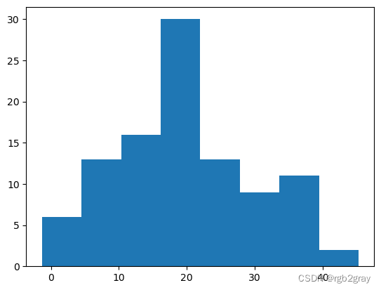
![在这里插入图片描述](https://img-blog.csdnimg.cn/direct/8ceeaaebbdc74efabf2c640a0950a1a6.png)

print("Population mean is:", np.mean(data))

print("Population variance is:", np.var(data))

Population mean is: 19.73510302232665
Population variance is: 105.44761217481347

#One sample with 30 numbers, this is what we have in hand.

sample_30 = np.random.choice(data, 30, replace=True)

sample_30

array([30.84743651, 39.13238623, 34.37879933, 13.32946651, 13.69039686,
        9.1263876 ,  6.87104071, 31.79246417, 10.98409074, 18.58904375,
       18.87102583, 10.23985703, 13.59549372, 25.24450873, 26.42390427,
        5.08193247, 31.79246417, 28.92760549, 15.4169132 ,  8.71363322,
        7.00419646, 25.26497935,  5.51315604, 22.28515871, 15.15546063,
       30.84743651, 24.14380325, 13.98657903, 25.24450873,  0.90316588])

1.构建Bootstrap CI

#Define a bootstrap function:
def bootstrap(sample):
    
    bootstrap_mean_list = []
    
    for i in range(10000):
        #generate a re-sample with the original sample size, with replacement
        subsample = np.random.choice(sample, len(sample), replace=True)
        
        #compute sub-sample mean
        subsample_mean = np.mean(subsample)

        bootstrap_mean_list.append(subsample_mean)
    
    #Calculatet the mean and std of the bootstrap sampling distribution
    bootstrap_mean = np.mean(bootstrap_mean_list)
    boostrap_std = np.std(bootstrap_mean_list)
    
    # mean +- 2*std for an approximate 95% CI.
    CI = [(bootstrap_mean - 2*boostrap_std), (bootstrap_mean + 2*boostrap_std)]
    
    return CI,bootstrap_mean_list

#Do the same thing for the percentile-based method:
def bootstrap_perc(sample):
    
    bootstrap_mean_list = []
    
    for i in range(1000):
        #generate a re-sample with the original sample size, with replacement
        subsample = np.random.choice(sample, len(sample), replace=True)
        
        #compute sample mean
        subsample_mean = np.mean(subsample)

        bootstrap_mean_list.append(subsample_mean)
    
    #Get the lower and upper bound for the middle 95%:
    percentile_CI = [np.percentile(bootstrap_mean_list, 2.5), 
          np.percentile(bootstrap_mean_list, 97.5)]
    
    return percentile_CI,bootstrap_mean_list

#Define a anlytical based function:
def anlytical(sample):
    
    sample_mean = np.mean(sample)
    
    err_of_margin = 2*np.std(sample)/np.sqrt(len(sample))
    
    # mean +- 2*std for an approximate 95% CI.
    CI_lower = sample_mean - err_of_margin
    CI_upper = sample_mean + err_of_margin
    
    CI = [CI_lower, CI_upper]
    
    return CI

比较引导 CI 与分析 CI：

bootstrap_CI, bootstrap_mean_list = bootstrap(sample_30)
bootstrap_CI_perc, bootstrap_mean_list_perc = bootstrap_perc(sample_30)
analytical_CI = anlytical(sample_30)

print("95% analytical CI: ", analytical_CI)
print("95% bootstrap CI: ", bootstrap_CI)
print("95% percentile-based bootstrap CI: ", bootstrap_CI_perc)

95% analytical CI:  [15.105707709695746, 22.45411196607375]
95% bootstrap CI:  [15.166149117216644, 22.429589185859715]
95% percentile-based bootstrap CI:  [15.128839804780965, 22.302901561304623]

测试 95% CI 的覆盖率

引导程序
基于百分位数的 Bootstrap
分析

%%time
#generate samples for multiple times
counter = 0
counter_perc = 0
true_mean = np.mean(data)

for i in range(1000):
    #generate a sample with 30 numbers
    sample = np.random.choice(data, 30, replace=True)
    
    #For each sample, we compute the two CIs:
    ci,_ = bootstrap(sample)
    perc_ci,_ = bootstrap_perc(sample)
    analytical_ci = anlytical(sample)
    
    #Check the coverage
    if ci[0] <= true_mean <= ci[1]:
        counter = counter + 1
        
    if perc_ci[0] <= true_mean <= perc_ci[1]:
        counter_perc = counter_perc + 1

CPU times: total: 28.3 s
Wall time: 2min 6s

print("Number of times 95% bootstrap CI covered the population mean:", 
      counter,"out of 1000")

Number of times 95% bootstrap CI covered the population mean: 944 out of 1000

print("Number of times 95% percentile-based bootstrap CI covered the population mean:", 
      counter,"out of 1000")

Number of times 95% percentile-based bootstrap CI covered the population mean: 944 out of 1000

print("Number of times 95% analytical CI covered the population mean:", 
      counter,"out of 1000")

Number of times 95% analytical CI covered the population mean: 944 out of 1000

相关系数的 Bootstrap 置信区间

import pandas as pd
url = 'https://raw.githubusercontent.com/mwaskom/seaborn-data/master/mpg.csv'
df = pd.read_csv(url)
df = df.dropna()

from scipy.stats import *

plt.scatter(df.horsepower, df.acceleration)
plt.xlabel("Horsepower")
plt.ylabel("Acceleration")

d:\work\miniconda3\lib\site-packages\scipy\__init__.py:146: UserWarning: A NumPy version >=1.16.5 and <1.23.0 is required for this version of SciPy (detected version 1.23.3
  warnings.warn(f"A NumPy version >={np_minversion} and <{np_maxversion}"





Text(0, 0.5, 'Acceleration')

在这里插入图片描述

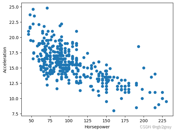
print("Pearson:",pearsonr(df.horsepower, df.acceleration))

Pearson: (-0.6891955103342369, 1.5818862297814436e-56)

sample_car = df.sample(frac=0.3,replace=True)
sample_car

	mpg	cylinders	displacement	horsepower	weight	acceleration	model_year	origin	name
238	33.5	4	98.0	83.0	2075	15.9	77	usa	dodge colt m/m
194	22.5	6	232.0	90.0	3085	17.6	76	usa	amc hornet
380	36.0	4	120.0	88.0	2160	14.5	82	japan	nissan stanza xe
142	26.0	4	79.0	67.0	1963	15.5	74	europe	volkswagen dasher
312	37.2	4	86.0	65.0	2019	16.4	80	japan	datsun 310
...	...	...	...	...	...	...	...	...	...
271	23.2	4	156.0	105.0	2745	16.7	78	usa	plymouth sapporo
136	16.0	8	302.0	140.0	4141	14.0	74	usa	ford gran torino
332	29.8	4	89.0	62.0	1845	15.3	80	europe	vokswagen rabbit
272	23.8	4	151.0	85.0	2855	17.6	78	usa	oldsmobile starfire sx
85	13.0	8	350.0	175.0	4100	13.0	73	usa	buick century 350

118 rows × 9 columns

print("Pearson:",pearsonr(sample_car.horsepower, sample_car.acceleration))

Pearson: (-0.7670736293678354, 4.176876123725007e-24)

#Define a bootstrap function:
np.random.seed(222)
def bootstrap_pearson(sample_car):
    
    bootstrap_cor_list = []
    
    for i in range(10000):
        #generate a re-sample with the original sample size, with replacement
        subsample = sample_car.sample(len(sample), replace=True)
        
        #compute correlation
        sample_cor = pearsonr(subsample.horsepower, subsample.acceleration)[0]

        bootstrap_cor_list.append(sample_cor)
    
    #Get the lower and upper bound for the middle 95%:
    percentile_CI = [np.percentile(bootstrap_cor_list, 2.5), 
          np.percentile(bootstrap_cor_list, 97.5)]
    
    return percentile_CI

bootstrap_pearson(sample_car)

[-0.897486157722385, -0.49473536389623324]

print("95% confidence interval of the Pearson correlation coefficient is:",
     "[-0.855 to -0.606]")

95% confidence interval of the Pearson correlation coefficient is: [-0.855 to -0.606]

我们有 95% 的信心认为人群中 HP 和 ACC 的真实相关性在 -0.855 到 -0.606 之间。

在这种情况下，CI 不覆盖 0，这意味着总体相关系数不为零。因此，我们从样本中观察到的负趋势不仅仅是因为抽样变化，而是因为总体中真正的相关性是负的。
_cor_list, 97.5)]

return percentile_CI



```python
bootstrap_pearson(sample_car)

[-0.897486157722385, -0.49473536389623324]

print("95% confidence interval of the Pearson correlation coefficient is:",
     "[-0.855 to -0.606]")

95% confidence interval of the Pearson correlation coefficient is: [-0.855 to -0.606]

我们有 95% 的信心认为人群中 HP 和 ACC 的真实相关性在 -0.855 到 -0.606 之间。

在这种情况下，CI 不覆盖 0，这意味着总体相关系数不为零。因此，我们从样本中观察到的负趋势不仅仅是因为抽样变化，而是因为总体中真正的相关性是负的。

2.统计推断置信区间

本笔记本演示了估计的置信区间 (CI) 的概念。我们将检查 CI 的覆盖概率。

考虑这样一个场景：FSU 有 20,000 名学生，他们的智商水平服从正态分布，平均值为 110，标准差为 10。让我们从学生群体中抽取样本，并检查样本与总体之间的关系。

import numpy as np
import matplotlib.pyplot as plt

生成人口数据

N = 20000 #20,000 students

#Generate from a normal distribution
data = np.random.randn(N)*10 + 110

plt.hist(data)

(array([  48.,  288., 1185., 3287., 5481., 5239., 3162., 1050.,  230.,
          30.]),
 array([ 73.30451127,  80.71913869,  88.13376612,  95.54839355,
        102.96302097, 110.3776484 , 117.79227582, 125.20690325,
        132.62153068, 140.0361581 , 147.45078553]),
 <BarContainer object of 10 artists>)

在这里插入图片描述

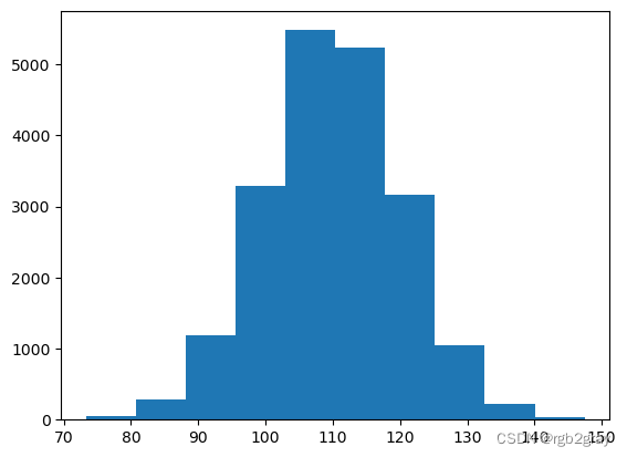
print("Population mean is:", np.mean(data))
print("Population variance is:", np.var(data))

Population mean is: 110.01962672036136
Population variance is: 102.25452537436367

现在让我们抽取样本。让我们从 10 名学生的样本开始

#One sample with 10 numbers

sample_10 = np.random.choice(data, 10)

sample_10

array([109.62388683,  91.97729472, 100.46429321, 111.00988364,
       108.31788058, 113.66683355, 109.74268367, 113.06416223,
       105.39076392, 122.01725268])

print("The sample mean is: ", np.mean(sample_10))

The sample mean is:  108.52749350347217

如果我们重复采样过程（例如 1,000 次）怎么样？

从 t 分布获取临界 t 值。自由度：10-1（样本大小 - 1）。置信区间宽度：95%。

from scipy import stats

t = stats.t.ppf(1-0.05/2, 9)
print(t)

d:\work\miniconda3\lib\site-packages\scipy\__init__.py:146: UserWarning: A NumPy version >=1.16.5 and <1.23.0 is required for this version of SciPy (detected version 1.23.3
  warnings.warn(f"A NumPy version >={np_minversion} and <{np_maxversion}"


2.2621571627409915

coverage_list = []

for i in range(1000):
    #generate a sample with 10 numbers
    sample = np.random.choice(data, 10)
    
    #compute sample mean
    sample_mean = np.mean(sample)
    
    err_of_margin = t*np.std(sample)/np.sqrt(10)
    
    CI_lower = sample_mean - err_of_margin
    CI_upper = sample_mean + err_of_margin
    
    true_mean = np.mean(data)
    
    is_covered = (true_mean>=CI_lower) and (true_mean<=CI_upper)
    
    print(i," 95% confidence interval ", [CI_lower, CI_upper], "Cover the true mean?", is_covered)
    
    coverage_list.append(is_covered)

0  95% confidence interval  [102.7151079840605, 118.2405606324954] Cover the true mean? True
1  95% confidence interval  [104.23885267719237, 118.10221181506196] Cover the true mean? True
2  95% confidence interval  [103.72346627181192, 115.9391835906615] Cover the true mean? True
3  95% confidence interval  [104.62550349440005, 115.14252771113254] Cover the true mean? True
4  95% confidence interval  [102.12727319514039, 112.16268597210077] Cover the true mean? True
5  95% confidence interval  [101.08352856103731, 118.69180761678739] Cover the true mean? True
6  95% confidence interval  [103.18857595332162, 113.00591633235916] Cover the true mean? True
7  95% confidence interval  [103.55533372607188, 110.30496134366432] Cover the true mean? True
8  95% confidence interval  [90.18976464492026, 103.9824575401898] Cover the true mean? False
9  95% confidence interval  [102.14358563332436, 115.72116848794366] Cover the true mean? True
10  95% confidence interval  [100.80227845656053, 111.93303378484153] Cover the true mean? True
11  95% confidence interval  [103.89446446670988, 114.34313482587856] Cover the true mean? True
12  95% confidence interval  [100.7487394903015, 111.36109764079389] Cover the true mean? True

3.统计推断点估计

本笔记本演示了统计量抽样分布的概念。这也表明

样本均值是无偏的
样本方差是无偏的
均值和方差抽样变异的解析解

样本平均值

import numpy as np
import matplotlib.pyplot as plt

生成人口数据

N = 20000 #20,000 students

#Generate from a normal distribution
data = np.random.randn(N)*10 + 110

plt.hist(data)

(array([   8.,  142.,  843., 3136., 5751., 5935., 3176.,  867.,  127.,
          15.]),
 array([ 69.32483145,  77.45863551,  85.59243958,  93.72624364,
        101.8600477 , 109.99385177, 118.12765583, 126.26145989,
        134.39526396, 142.52906802, 150.66287208]),
 <BarContainer object of 10 artists>)

在这里插入图片描述

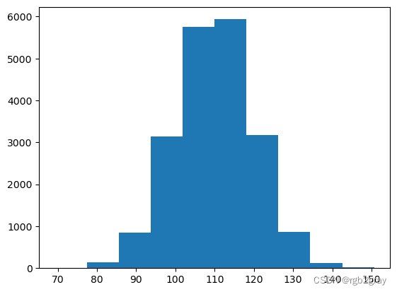
print("Population mean is:", np.mean(data))
print("Population variance is:", np.var(data))

Population mean is: 110.07413289511938
Population variance is: 98.89323295421896

现在让我们抽取样本。让我们从 10 名学生的样本开始

#One sample with 10 numbers

sample_10 = np.random.choice(data, 10)

sample_10

array([111.66777512, 112.16222242, 118.08689454, 110.24523641,
       125.48603522,  88.41367076, 125.67988677, 113.88800138,
       108.6807358 , 121.01857026])

print("The sample mean is: ", np.mean(sample_10))

The sample mean is:  113.53290286905217

如果我们重复采样过程（例如 1,000 次）怎么样？

#Create an empty list to hold the numbers from each sample
sample_10_mean_list = []

for i in range(1000):
    #generate a sample with 10 numbers
    sample = np.random.choice(data, 10)
    
    #compute sample mean
    sample_mean = np.mean(sample)
    
    print(i," sample mean: ", sample_mean)
    
    #append them to the list
    sample_10_mean_list.append(sample_mean)

0  sample mean:  108.17391918529407
1  sample mean:  111.67818693824806
2  sample mean:  111.67822497907324
3  sample mean:  107.24418829414785
4  sample mean:  113.17329723752623
5  sample mean:  112.9070413608591
6  sample mean:  108.04910734829619
7  sample mean:  112.5903576727253
8  sample mean:  113.62852862972878
9  sample mean:  113.27149334572691
10  sample mean:  107.76969738534706
11  sample mean:  109.1620666792978
12  sample mean:  103.71358812699627
13  sample mean:  107.697395964914
14  sample mean:  110.8082408750503
15  sample mean:  110.92158184257207
16  sample mean:  108.58419010871549
17  sample mean:  109.65230764397218
18  sample mean:  109.86678913378717
19  sample mean:  105.08768958694495
20  sample mean:  106.88640190007649
21  sample mean:  112.56008138539062
22  sample mean:  110.83395797118828
23  sample mean:  110.73008027594503
24  sample mean:  109.3294505313664
25  sample mean:  110.04042595076564
26  sample mean:  109.67050530705797
27  sample mean:  108.32738807341839
28  sample mean:  108.49314412381798
29  sample mean:  107.1858761872827
30  sample mean:  112.46187853160286
31  sample mean:  113.12349039970186
32  sample mean:  110.14207252003163
33  sample mean:  110.75599034550528
34  sample mean:  106.8240410457283
35  sample mean:  111.8765477301838
36  sample mean:  113.82299698648565
37  sample mean:  109.31286148365352
38  sample mean:  111.97700620796886
39  sample mean:  109.9008197839028
40  sample mean:  107.69013776731724
41  sample mean:  114.28574317155494
42  sample mean:  109.50146395888653
43  sample mean:  107.40447023607123
44  sample mean:  116.24621309981323
45  sample mean:  112.67872689503027
46  sample mean:  106.53331942661855
47  sample mean:  110.35618578397953
48  sample mean:  107.67531638860439
49  sample mean:  111.03510449989963
50  sample mean:  109.03305491756535
51  sample mean:  111.12749226215763
52  sample mean:  107.44884335343575
53  sample mean:  111.4216569660086
54  sample mean:  112.14976633180977
55  sample mean:  108.046169949935
56  sample mean:  107.78856332959371
57  sample mean:  115.0407995071375
58  sample mean:  107.82026621773139
59  sample mean:  106.80442741389179
60  sample mean:  109.07177961379848
61  sample mean:  110.57205199833035
62  sample mean:  107.35628147704801
63  sample mean:  107.84236667449561
64  sample mean:  111.90515735465651
65  sample mean:  114.4823745877502
66  sample mean:  102.21096088759352
67  sample mean:  112.18457688111475
68  sample mean:  107.4440654002789
69  sample mean:  108.47620386204194
70  sample mean:  115.00823605453897
71  sample mean:  106.75913949864893
72  sample mean:  111.13852427880879
73  sample mean:  108.95844954274037
74  sample mean:  113.59768517919773
75  sample mean:  111.31910512168243
76  sample mean:  106.38067170844681
77  sample mean:  109.49375945640797
78  sample mean:  115.093047567975
79  sample mean:  106.09833252432466
80  sample mean:  116.4311422319212
81  sample mean:  108.28528941038228
82  sample mean:  103.82927317186042
83  sample mean:  111.18673783032439
84  sample mean:  108.4971016336932
85  sample mean:  105.49599715374734
86  sample mean:  110.14529385508467
87  sample mean:  105.75197161089457
88  sample mean:  115.80545357784479
89  sample mean:  107.75685400068934
90  sample mean:  109.49381609427321
91  sample mean:  108.95402323987977
92  sample mean:  111.97213167688433
93  sample mean:  109.47712760468328
94  sample mean:  113.14660304988516
95  sample mean:  110.80976482820472
96  sample mean:  107.92343270315664
97  sample mean:  108.37770599789269
98  sample mean:  105.25528550623233
99  sample mean:  115.05666095395479
100  sample mean:  107.77247710607735
101  sample mean:  108.89543987766524
102  sample mean:  112.12273016811253
103  sample mean:  114.80392467210928
104  sample mean:  106.68961413411903
105  sample mean:  106.03545032270267
106  sample mean:  114.97887048765503
107  sample mean:  110.37581153007821
108  sample mean:  110.65923878869683
109  sample mean:  111.3430788040037
110  sample mean:  107.7232254285943
111  sample mean:  111.57244948737664
112  sample mean:  105.28194979231736
113  sample mean:  109.98995161589244
114  sample mean:  109.53396064067333
115  sample mean:  111.38428386596779
116  sample mean:  110.97486991904695
117  sample mean:  112.87118032789704
118  sample mean:  108.04167623331617
119  sample mean:  109.74945215273877
120  sample mean:  113.34034390095641
121  sample mean:  108.87412423611276
122  sample mean:  105.06601270840356
123  sample mean:  109.90153164811923
124  sample mean:  108.29931093364205
125  sample mean:  114.54952533305318
126  sample mean:  108.41885224159255
127  sample mean:  109.432696156925
128  sample mean:  108.85548860855647
129  sample mean:  106.69453432738733
130  sample mean:  110.73156301741199
131  sample mean:  110.3344293210414
132  sample mean:  106.43368100363816
133  sample mean:  111.57845827640968
134  sample mean:  116.41696101920373
135  sample mean:  110.09786113805441
136  sample mean:  110.12713022826912
137  sample mean:  115.19539623223059
138  sample mean:  114.69947911209549
139  sample mean:  112.15932563335575
140  sample mean:  105.03670120615747
141  sample mean:  106.55324659192142
142  sample mean:  108.87155226347852
143  sample mean:  113.19328040597836
144  sample mean:  107.43749597783346
145  sample mean:  112.52280142597355
146  sample mean:  104.25237526935716
147  sample mean:  111.74730695830422
148  sample mean:  106.47421562458676
149  sample mean:  110.41192960632631
150  sample mean:  111.06560448474977
151  sample mean:  110.8574597363748
152  sample mean:  113.5702179737926
153  sample mean:  102.94360945489191
154  sample mean:  112.51717223500005
155  sample mean:  116.24740871295299
156  sample mean:  113.38278417361005
157  sample mean:  115.25751695567212
158  sample mean:  110.0492555852654
159  sample mean:  111.79273879730708
160  sample mean:  115.00085251159253
161  sample mean:  108.46956146896632
162  sample mean:  112.25352540521085
163  sample mean:  110.09704245884075
164  sample mean:  109.37142519972653
165  sample mean:  113.528730214851
166  sample mean:  111.73192964440406
167  sample mean:  107.83625790041121
168  sample mean:  110.30771604129515
169  sample mean:  104.20621128051827
170  sample mean:  110.32212617511611
171  sample mean:  108.00438566363746
172  sample mean:  113.61660167443861
173  sample mean:  108.81058515088898
174  sample mean:  110.77800251434556
175  sample mean:  113.10422375502681
176  sample mean:  114.39592439664179
177  sample mean:  112.55187994163687
178  sample mean:  107.23704574273629
179  sample mean:  108.57205135565349
180  sample mean:  110.58745831308568
181  sample mean:  110.47926496421303
182  sample mean:  107.99057552600043
183  sample mean:  114.1629001335393
184  sample mean:  106.45733896312565
185  sample mean:  114.21043571521477
186  sample mean:  111.0160001995882
187  sample mean:  110.23687892814004
188  sample mean:  113.88730941650071
189  sample mean:  107.42852295711978
190  sample mean:  109.50077760121633
191  sample mean:  110.37270694898527
192  sample mean:  105.7880522406582
193  sample mean:  114.6503862528984
194  sample mean:  109.42960390312935
195  sample mean:  104.93643110081601

每次采样时我们都会观察到不同的样本均值。如果我们看一下它们的分布，样本均值的抽样分布是：

plt.hist(sample_10_mean_list)

(array([  9.,  18.,  71., 148., 220., 207., 164., 105.,  49.,   9.]),
 array([100.41739832, 102.22911703, 104.04083574, 105.85255445,
        107.66427316, 109.47599187, 111.28771058, 113.0994293 ,
        114.91114801, 116.72286672, 118.53458543]),
 <BarContainer object of 10 artists>)

在这里插入图片描述

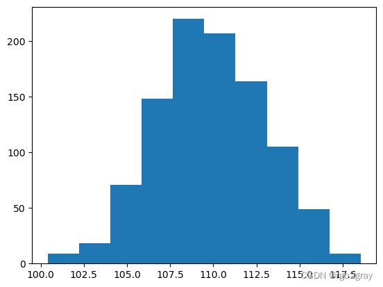
**重要提示：**这不是智商水平的分布！这是给定样本（样本中有 10 名学生）的平均 IQ 水平超过 1,000 次的分布。

该分布的平均值为：

np.mean(sample_10_mean_list)

109.81834080140132

让我们与总体平均值进行比较：

np.mean(data)

110.07413289511938

相当接近！

如果我们1）增加样本量（10->100），样本均值是否会更接近真实均值？ 2) 进行更多采样（10,000 -> 1,000,000）。是的！

#Create an empty list to hold the numbers from each sample
sample_100_mean_list = []

for i in range(1000000):
    #generate a sample with 100 numbers
    sample = np.random.choice(data, 100)
    
    #compute sample mean
    sample_mean = np.mean(sample)
    
    #print(i," sample mean: ", sample_mean)
    
    #append them to the list
    sample_100_mean_list.append(sample_mean)

plt.hist(sample_100_mean_list)

(array([6.80000e+01, 2.14900e+03, 2.68310e+04, 1.42865e+05, 3.29388e+05,
        3.28362e+05, 1.41841e+05, 2.63350e+04, 2.09200e+03, 6.90000e+01]),
 array([105.35779164, 106.30191012, 107.24602861, 108.1901471 ,
        109.13426558, 110.07838407, 111.02250256, 111.96662104,
        112.91073953, 113.85485802, 114.7989765 ]),
 <BarContainer object of 10 artists>)

在这里插入图片描述

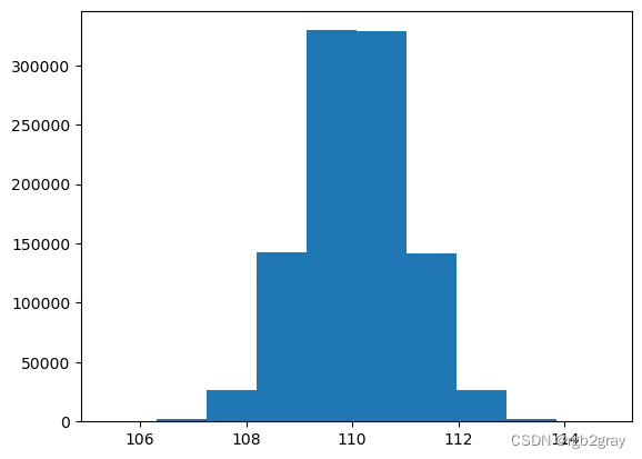
print("Average sample mean:", np.mean(sample_100_mean_list))
print("True mean:", np.mean(data))

Average sample mean: 110.07524696756842
True mean: 110.07413289511938

进一步增加样本量和样本次数将使样本均值收敛于真实总体均值，这表明样本均值是一个无偏统计量。

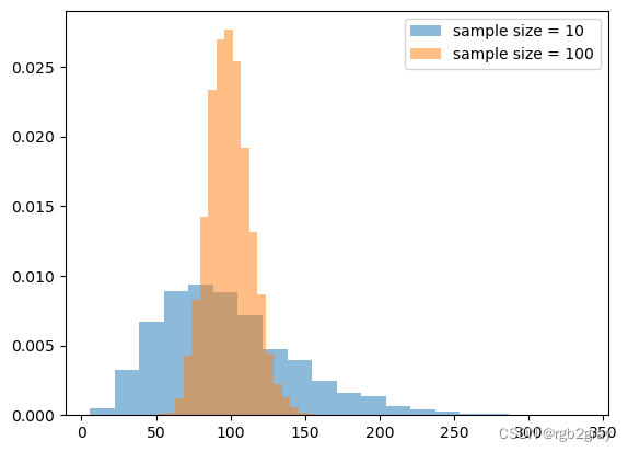
我们可以比较使用两个不同样本量时样本均值的分布。

plt.hist(sample_10_mean_list, density=True, alpha=0.5,bins=10,label='sample size = 10')

plt.hist(sample_100_mean_list, density=True, alpha=0.5,bins=10,label='sample size = 100')

plt.legend()

<matplotlib.legend.Legend at 0x1a70b3b9a90>

在这里插入图片描述

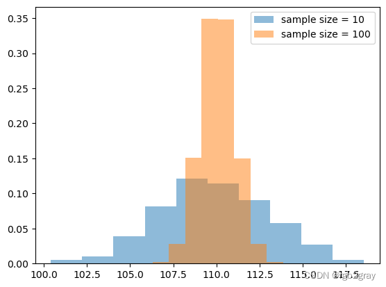
当样本量较小时，抽样分布更宽（即抽样变异性更大）！

这是因为：从分析上来说，样本均值的抽样分布遵循正态分布，均值为总体均值，标准差为： $\frac{\sigma}{\sqrt{n}}$

其中 $\sigma$ 是总体标准差， $n$ 是样本量。

print("Analytical SD of the sampling distribution:", 
      np.std(data)/np.sqrt(10))

print("Empirical SD of the sampling distribution:", 
      np.std(sample_10_mean_list))

Analytical SD of the sampling distribution: 3.1447294470942797
Empirical SD of the sampling distribution: 3.1421107844908382

print("Analytical SD of the sampling distribution:", 
      np.std(data)/np.sqrt(100))

print("Empirical SD of the sampling distribution:", 
      np.std(sample_100_mean_list))

Analytical SD of the sampling distribution: 0.9944507677819902
Empirical SD of the sampling distribution: 0.994316399287971

同样，让我们检查样本方差的抽样分布。

#define a small function to calculate sample variance.
def sample_var(sample):
    mean = np.mean(sample)
    n = sample.shape[0]
    return np.sum((sample - mean)**2)/(n-1)

#One sample with 10 numbers

sample_10 = np.random.choice(data, 10)

sample_10

array([121.64683719, 103.11098717, 116.80834819, 103.55885849,
        91.93607486, 110.61085577, 120.87592219, 101.59268352,
       117.57011851, 108.56843983])

print("Sample variance is:", sample_var(sample_10))

Sample variance is: 93.84088686288874

#generate samples for multiple times
sample_10_variance_list = []

for i in range(10000):
    #generate a sample with 10 numbers
    sample = np.random.choice(data, 10)
    
    #compute sample variance
    sample_variance = sample_var(sample)
    
    print(i," sample variance: ", sample_variance)
    
    #append them to the list
    sample_10_variance_list.append(sample_variance)

0  sample variance:  133.16255153634953
1  sample variance:  84.95111363055562
2  sample variance:  129.25853520691152
3  sample variance:  162.9507939120388
4  sample variance:  57.65250685184362
5  sample variance:  127.05245098320125
6  sample variance:  70.03273515311018
7  sample variance:  96.41498645686788
8  sample variance:  83.05696382116894
9  sample variance:  119.12242739103021
10  sample variance:  72.61720603700626

方差的抽样分布

plt.hist(sample_10_variance_list)

(array([9.170e+02, 3.058e+03, 3.017e+03, 1.754e+03, 8.010e+02, 2.870e+02,
        1.000e+02, 5.400e+01, 9.000e+00, 3.000e+00]),
 array([  8.95012759,  45.1402609 ,  81.3303942 , 117.5205275 ,
        153.71066081, 189.90079411, 226.09092741, 262.28106072,
        298.47119402, 334.66132733, 370.85146063]),
 <BarContainer object of 10 artists>)

在这里插入图片描述

print("Average of sample variance:", np.mean(sample_10_variance_list))

print("True variance:", np.var(data))

Average of sample variance: 99.59784954844092
True variance: 98.89323295421896

再次，相当接近！

增加样本大小和样本数量：

#generate samples for multiple times
sample_100_variance_list = []

for i in range(1000000):
    #generate a sample with 100 numbers
    sample = np.random.choice(data, 100)
    
    #compute sample variance
    sample_variance = sample_var(sample)
    
    #append them to the list
    sample_100_variance_list.append(sample_variance)

print("Average of sample variance:", np.mean(sample_100_variance_list))
print("True variance:", np.var(data))

Average of sample variance: 98.88787841866694
True variance: 98.89323295421896

靠近点！

比较两个相同大小的样本均值的抽样分布。

plt.hist(sample_10_variance_list,density=True,alpha=0.5,bins=20,label='sample size = 10')
plt.hist(sample_100_variance_list,density=True,alpha=0.5,bins=20,label='sample size = 100')
plt.legend()

<matplotlib.legend.Legend at 0x1a701f14670>

在这里插入图片描述

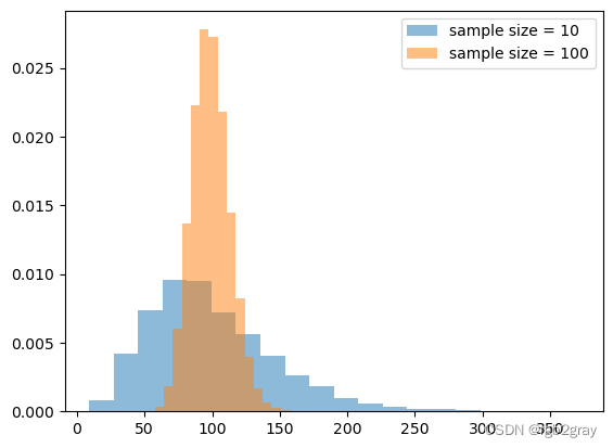
从分析上看，样本方差的抽样分布遵循自由度为 n - 1（n 为样本大小）的卡方分布。

$(n-1)s^2/\sigma^2 \sim \chi^2_{n-1}$

其中 $s$ 是样本标准差， $\sigma$ 是总体标准差

numpy 函数模拟卡方分布：random.chisquare(df, size=None)

anlytical_dist_10 = np.random.chisquare(10-1, 10000)*np.var(data)/(10-1)

anlytical_dist_100 = np.random.chisquare(100-1, 10000)*np.var(data)/(100-1)

plt.hist(anlytical_dist_10,density=True,alpha=0.5,bins=20,label='sample size = 10')
plt.hist(anlytical_dist_100,density=True,alpha=0.5,bins=20,label='sample size = 100')
plt.legend()

<matplotlib.legend.Legend at 0x1a711da2190>

在这里插入图片描述

分析分布与我们的经验抽样分布相同！

Applied Spatial Statistics（一）统计推断

Applied Spatial Statistics（一）统计推断

1.统计推断：Bootstrap 置信区间

2.统计推断置信区间

现在让我们抽取样本。 让我们从 10 名学生的样本开始

如果我们重复采样过程（例如 1,000 次）怎么样？

3.统计推断点估计

样本平均值

现在让我们抽取样本。 让我们从 10 名学生的样本开始

如果我们重复采样过程（例如 1,000 次）怎么样？

同样，让我们检查样本方差的抽样分布。

现在让我们抽取样本。让我们从 10 名学生的样本开始

现在让我们抽取样本。让我们从 10 名学生的样本开始