


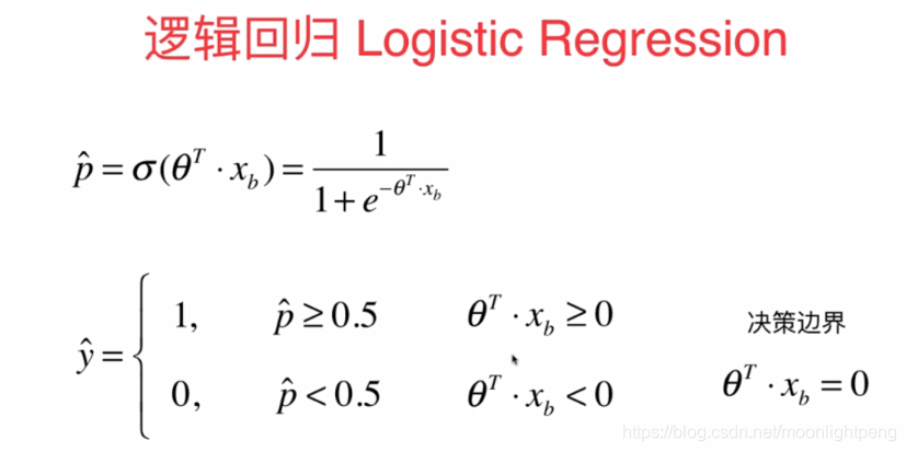
逻辑回归 Logistic Regression
-
解决分类问题
-
通常做分类算法,只能作二分法
-
sigmod(x) = 1 / (1+e^-t)
# 直线型逻辑回归
from sklearn.linear_model import LogisticRegression
log_reg = LogisticRegression()
log_reg.fit(x_train, y_train)
log_reg.score(x_test, y_test)

# 多项式逻辑回归
from sklearn.preprocessing import PolynomialFeatures  # 先使用poly处理x
from sklearn.pipeline import Pipeline
from sklearn.preprocessing import StandardScaler

log_reg_pipe = Pipeline([
    ('poly', PolynomialFeatures(degree=2)),
    ('Standard', StandardScaler()),
    ('log_reg', LogisticRegression())
])
log_reg_pipe.fit(x_train, y_train)
log_reg_pipe.score(x_test, y_test)
分类准确度问题
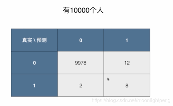
- 对数据极度偏斜,只使用分类准确度远远不够
- 癌症的预测准确度为99.99%,但是只有0.01%的发病率,则对大多数人基本上不用预测都是健康的,预测机制几乎失灵
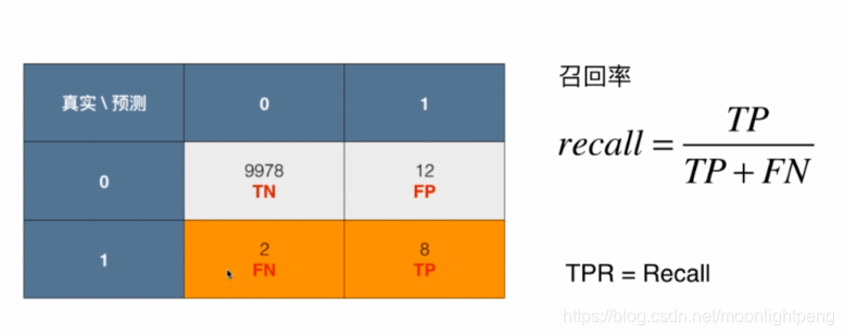
混淆矩阵 Confusion Matrix
- 行代表真实值,列代表预测值
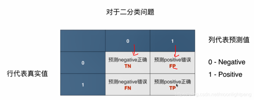
预测准确的有(0,0)(1,1),其余的都是预测错误的点
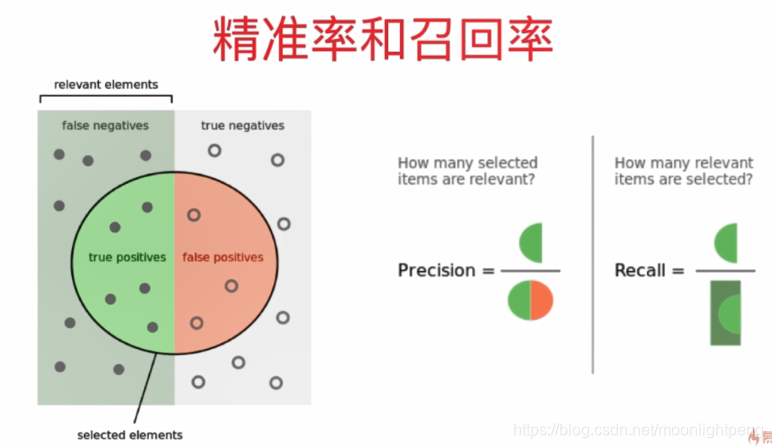
- 精准率:
precision = TP/ (TP + FP)只看对癌症预测成功或不成功的部分,而不对健康人群预测,健康人群的偏差过大 - 召回率:
recall = TP/ (TP + FN)对真实发生的癌症人群,能够发现的概率
from sklearn.metrics import confusion_matrix  # 引入混淆矩阵
confusion_matrix(y_test, y_predict)

from sklearn.metrics import precision_score  # 计算精准率
precision_score(y_test, y_predict)

from sklearn.metrics import recall_score  # 计算召回率
recall_score(y_test, y_predict)
- 有时候我们会注重精准率:如股票预测
- 侧重召回率:病人诊断
调和平均值F1 Score
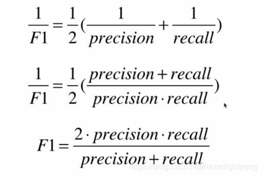
F1 = (2*precision * recall) / (precision + recall)
两个值如果有一个值偏小则整体偏小
两个都大时才大
对两个度量(精准率和召回率)的平衡计算
from sklearn.metrics import f1_score
f1_score(y_test, y_predict)
对数组值大于5的都变为1,小于5则为0
np.array(decision_scores >= 5, dtype='int')
Precision_Recall_Carve
- PR模型曲线更向外面积越大模型越好,
from sklearn.metrics import precision_recall_curve  # 引入准确率和召回率的曲线函数

precision, recall, thresholds = precision_recall_curve(y_test, dec_fun)  # 传入测试结果y_test和决策预测结果decision_function

print(precision.shape, recall.shape, thresholds.shape)  # threshold比其余的小一,故绘图时需要precision[:-1]

import matplotlib.pyplot as plt

plt.plot(thresholds, precision[:-1], color='r')    # 分别画出准确率和召回率的曲线
plt.plot(thresholds, recall[:-1], color='b')
plt.show()

plt.plot(recall, precision)   # 画出准确率和召回率之间关系的曲线
plt.show()
ROC
- TPR
- FPR
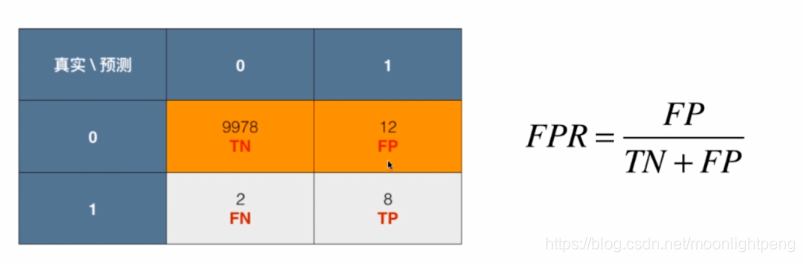
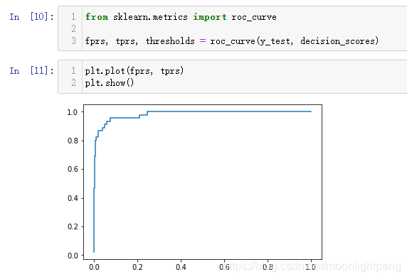
- 横轴为FPR, 纵轴为TPR,
plt.plot(fprs, tprs)
from sklearn.metrics import roc_curve
fprs, tprs, thresholds = roc_curve( y_test, dec_fun )   # 引入roc曲线
plt.plot(fprs, tprs)  # 绘制roc曲线
plt.show()

from sklearn.metrics import roc_auc_score   # 引入roc的曲线面积函数
roc_auc_score(y_test, dec_fun)   # 求出roc曲线面积
多分类问题
from sklearn.metrics import confusion_matrix
confusion_matrix(y_test, y_predict)     # 对分类问题中的混淆矩阵,此时y目标有多个特征值


 4万+
4万+

 被折叠的 条评论
为什么被折叠?
被折叠的 条评论
为什么被折叠?
 到【灌水乐园】发言


