多元线性回归

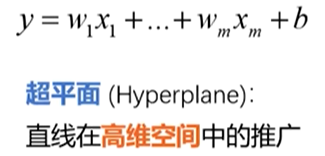
多元回归：回归分析中包括两个或两个以上的自变量。
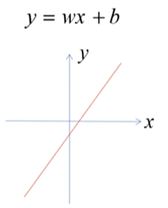
多元线性回归：因变量和自变量之间是线性关系。

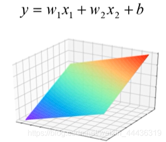
多元线性回归

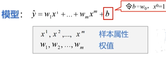
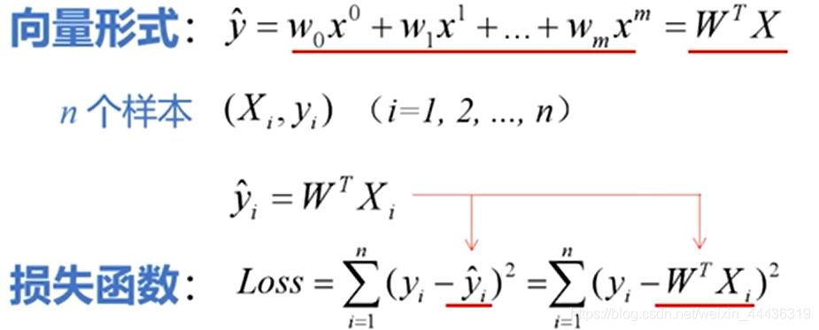
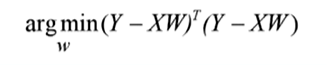
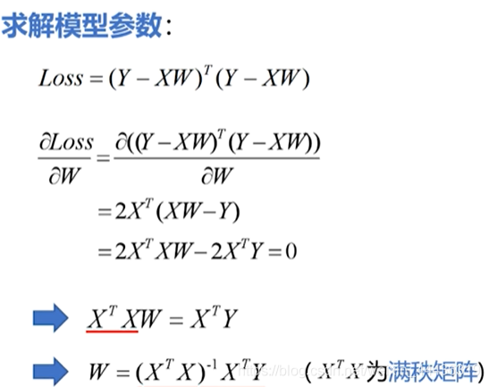
参数向量W取值要满足使Loss最小，由

可得到

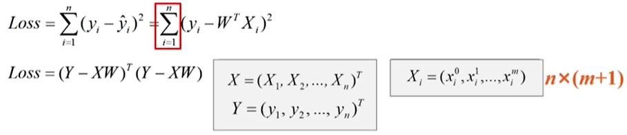
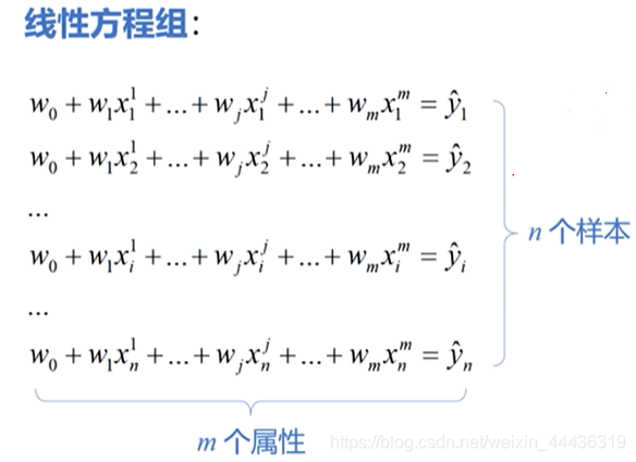
联立多个线性方程

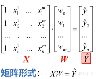
转化成矩阵形式

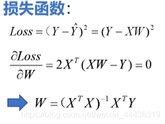
求解

代码实现

import tensorflow as tf
import numpy as np

#设置图像中显示中文
plt.rcParams['font.sans-serif'] = ['SimHei']
#房子面积
x1 = np.array([137.97,104.50,100.00,124.32,79.2,99.,124.,114.,106.69,138.05,53.75,46.91,68.,63.02,81.26,86.21])
x2 = np.array([3,2,2,3,1,2,3,2,2,3,1,1,1,1,2,2]) # 房间数
y = np.array([145.,110.,93.,116.,65.32,104.,118.,91.,62.,133.,51.,45.,78.5,69.65,75.69,95.3])# 价格
print(x1.shape,x2.shape,y.shape)
x0 = np.ones(len(x1))
X=np.stack((x0,x1,x2),axis=1)  # 把三个一维数组合并成一个二维数组
print(X)
Y = np.array(y).reshape(-1,1) #得到一个16维1列的二维数组

Xt = np.transpose(X) #计算X'
XtX_1 = np.linalg.inv(np.matmul(Xt,X)) # 计算(X'X)-1次方
XtX_1_Xt = np.matmul(XtX_1,Xt) # 计算(X'X)-1次方乘以X'
W = np.matmul(XtX_1_Xt,Y) #W=((X'X)-1次方)X'Y
W = W.reshape(-1)
print("多元线性回归方程：")
print("Y=",W[1],"*x1+",W[2],"*x2+",W[0])
print("请输入房屋面积和房间数，预测房屋销售价格：")
x1_test = float(input("商品房面积："))
x2_test = int(input("房间数："))

y_pred = W[1]*x1_test+W[2]*x2_test+W[0]
print("预测价格:",round(y_pred,2),"万元")

可视化

import numpy as np
import matplotlib.pyplot as plt
from mpl_toolkits.mplot3d import Axes3D

#设置图像中显示中文
plt.rcParams['font.sans-serif'] = ['SimHei']

x1 = np.array([137.97,104.50,100.00,124.32,79.2,99.,124.,114.,106.69,138.05,53.75,46.91,68.,63.02,81.26,86.21])
x2 = np.array([3,2,2,3,1,2,3,2,2,3,1,1,1,1,2,2])
y = np.array([145.,110.,93.,116.,65.32,104.,118.,91.,62.,133.,51.,45.,78.5,69.65,75.69,95.3])
print(x1.shape,x2.shape,y.shape)
x0 = np.ones(len(x1))
X=np.stack((x0,x1,x2),axis=1)  # 把三个一维数组合并成一个二维数组
print(X)
Y = np.array(y).reshape(-1,1) #得到一个16维1列的二维数组

Xt = np.transpose(X) #计算X'
XtX_1 = np.linalg.inv(np.matmul(Xt,X)) # 计算(X'X)-1次方
XtX_1_Xt = np.matmul(XtX_1,Xt) # 计算(X'X)-1次方乘以X'
W = np.matmul(XtX_1_Xt,Y) #W=((X'X)-1次方)X'Y
W = W.reshape(-1)
# print("多元线性回归方程：")
# print("Y=",W[1],"*x1+",W[2],"*x2+",W[0])
# print("请输入房屋面积和房间数，预测房屋销售价格：")
# x1_test = float(input("商品房面积："))
# x2_test = int(input("房间数："))
#
# y_pred = W[1]*x1_test+W[2]*x2_test+W[0]
# print("预测价格:",round(y_pred,2),"万元")
y_pred = W[1]*x1+W[2]*x2+W[0]

fig = plt.figure(figsize=(8,6))
ax3d = Axes3D(fig) # 创建3D绘图对象
# ax3d.view_init(elev=0,azim=-90) # 改变图形视角elev表示水平高度，azim表示水平旋转角度

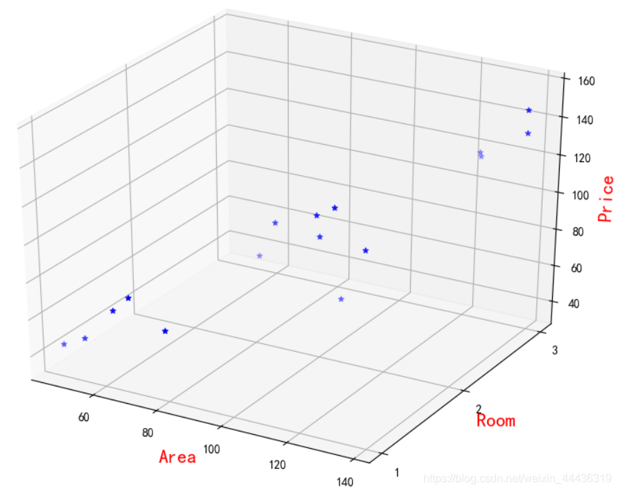
ax3d.scatter(x1,x2,y,color="b",marker="*")
ax3d.set_xlabel("Area",color="r",fontsize=16)
ax3d.set_ylabel("Room",color="r",fontsize=16)
ax3d.set_zlabel("Price",color="r",fontsize=16)
ax3d.set_yticks([1,2,3]) # 设置y轴的坐标轴刻度
ax3d.set_zlim3d(30,160) # 设置z轴的坐标轴范围


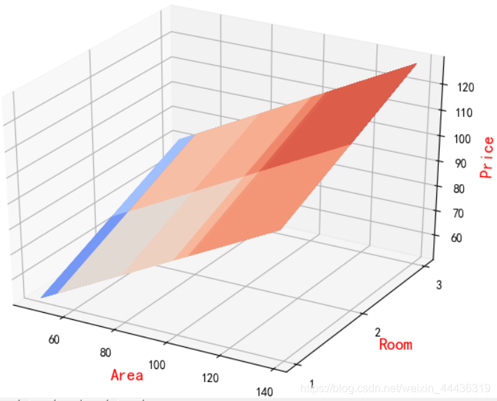
#绘制平面图
X1,X2 = np.meshgrid(x1,x2)
Y_PRED=W[0]+W[1]*X1+W[2]*X2

fig = plt.figure()
ax3d = Axes3D(fig)

ax3d.plot_surface(X1,X2,Y_PRED,cmap="coolwarm")

ax3d.set_xlabel("Area",color="r",fontsize=14)
ax3d.set_ylabel("Room",color="r",fontsize=14)
ax3d.set_zlabel("Price",color="r",fontsize=14)
ax3d.set_yticks([1,2,3])


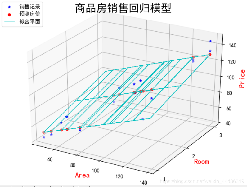
# 绘制散点图和线框图
plt.rcParams['font.sans-serif'] = ['SimHei']
fig = plt.figure()
ax3d = Axes3D(fig)

ax3d.scatter(x1,x2,y,color="b",marker="*",label="销售记录")
ax3d.scatter(x1,x2,y_pred,color="r",label="预测房价")
ax3d.plot_wireframe(X1,X2,Y_PRED,color="c",linewidth=0.5,label="拟合平面")

ax3d.set_xlabel("Area",color="r",fontsize=14)
ax3d.set_ylabel("Room",color="r",fontsize=14)
ax3d.set_zlabel("Price",color="r",fontsize=14)
ax3d.set_yticks([1,2,3])
plt.suptitle("商品房销售回归模型",fontsize=20)
plt.legend(loc="upper left")
plt.show()

结果