动手深度学习——Pytorch 入门语法一

持续更新ing

数据操作

import torch

x = torch.arange(12) # 创建⼀个⾏向量x。这个⾏向量包含从0开始的前12个整数
print(x.shape)  # 通过张量的shape属性来访问张量（沿每个轴的⻓度）的形状。
print(x.numel())  # 检查它的⼤小（size）

X = x.reshape(3,4)
print(X)
print(x.view(3,4))# 输出和上面一样。
# view()和reshape()功能一样，都可以改变张量形状。

z = torch.zeros((2,3,4)) # 全零张量
print(z)

z1 = torch.ones((2,3,4)) # 全1张量
print(z1)

randomNumber = torch.randn(3,4) # 创建⼀个形状为（3,4）的张量。其中的每个元素都从均值为0、标准差为1的标准⾼斯分布（正态分布）中随机采样

print(torch.tensor([[2, 1, 4, 3], [1, 2, 3, 4], [4, 3, 2, 1]])) # 给张量直接赋值

import torch

x= torch.tensor([1.0, 2, 4, 8])
y = torch.tensor([2,2,2,2])
print(x+y,x-y,x*y,x/y, x**y) # **运算符是求幂运算

print(torch.exp(x)) # 计算e的幂

X = torch.arange(12,dtype=torch.float32).reshape((3,4))
Y = torch.tensor([[2.0,1,4, 3],[1, 2, 3, 4], [4, 3, 2, 1]])

torch.cat((X,Y),dim=0) # 竖直连接，增加行。
torch.cat((X,Y),dim=1) # 横向连接，增加列

print(X == Y) # 结果为Ture 和 False

print(X.sum())  # 张量内元素求和
a = torch.arange(3).reshape((3,1))
b = torch.arange(2).reshape((1,2))

print(a,b)
print(a + b) # 沿着数组中⻓度为1的轴进⾏⼴播，矩阵a将复制列，矩阵b将复制⾏，然后再按元素相加。

print(X[-1],X[1:3]) # 索引和切片，与列表相似

X[1,2] = 9 # 指定索引来将元素写⼊矩阵。
print(X)

X[0:2,:] = 12 # 为多个元素赋值相同的值
print(X)


A =X.numpy() # 将深度学习框架定义的张量转换为NumPy张量（ndarray）
B = torch.tensor(A)
print(type(A), type(B))

a = torch.tensor([3.5])
print(a,a.item(), float(a), int(a)) #将⼤小为1的张量转换为Python标量

A = torch.arange(20).reshape((5,4))

print(A)
print(A.T) # 转置

A = torch.arange(20,dtype=torch.float32).reshape(5,4)
B = A.clone() # 通过分配新内存，将A的⼀个副本分配给B
print(A,A+B)

Tensor的合并与拆分

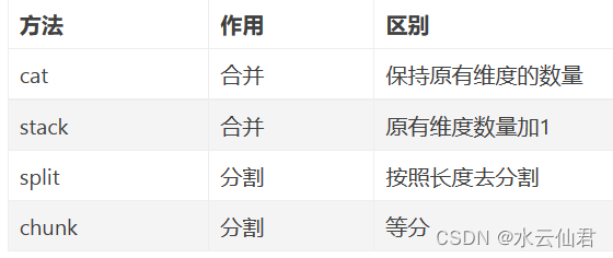
对于需要拼接的张量，维度数量必须相同，进行拼接的维度的尺寸可以不同，但是其它维度的尺寸必须相同。

>>> import torch
>>> x = torch.randn(2, 3)
>>> x
tensor([[-0.1997, -0.6900,  0.7039],
        [ 0.0268, -1.0140, -2.9764]])
>>> torch.cat((x, x, x), 0)	# 在 0 维(纵向)进行拼接，可以将一个张量序列进行合并。
tensor([[-0.1997, -0.6900,  0.7039],
        [ 0.0268, -1.0140, -2.9764],
        [-0.1997, -0.6900,  0.7039],
        [ 0.0268, -1.0140, -2.9764],
        [-0.1997, -0.6900,  0.7039],
        [ 0.0268, -1.0140, -2.9764]])
>>> torch.cat((x, x, x), 1)	# 在 1 维(横向)进行拼接
tensor([[-0.1997, -0.6900,  0.7039, -0.1997, -0.6900,  0.7039, -0.1997, -0.6900,
          0.7039],
        [ 0.0268, -1.0140, -2.9764,  0.0268, -1.0140, -2.9764,  0.0268, -1.0140,
         -2.9764]])
>>> y1 = torch.randn(5, 3, 6)
>>> y2 = torch.randn(5, 3, 6)
>>> torch.cat([y1, y2], 2).size()
torch.Size([5, 3, 12])
>>> torch.cat([y1, y2], 1).size()
torch.Size([5, 6, 6])

沿着一个新维度对输入张量序列进行连接。 序列中所有的张量都应该为相同形状

>>> x1 = torch.randn(2, 3)
>>> x2 = torch.randn(2, 3)
>>> torch.stack((x1, x2), 0).size()	# 在 0 维插入一个维度，进行区分拼接。也可以对一个张量序列进行拼接，即将多个相同维度的张量合并到一个高维度的张量中。
torch.Size([2, 2, 3])
>>> torch.stack((x1, x2), 1).size()	# 在 1 维插入一个维度，进行组合拼接
torch.Size([2, 2, 3])
>>> torch.stack((x1, x2), 2).size()
torch.Size([2, 3, 2])
>>> torch.stack((x1, x2), 0)
tensor([[[-0.3499, -0.6124,  1.4332],
         [ 0.1516, -1.5439, -0.1758]],

        [[-0.4678, -1.1430, -0.5279],
         [-0.4917, -0.6504,  2.2512]]])
>>> torch.stack((x1, x2), 1)
tensor([[[-0.3499, -0.6124,  1.4332],
         [-0.4678, -1.1430, -0.5279]],

        [[ 0.1516, -1.5439, -0.1758],
         [-0.4917, -0.6504,  2.2512]]])
>>> torch.stack((x1, x2), 2)
tensor([[[-0.3499, -0.4678],
         [-0.6124, -1.1430],
         [ 1.4332, -0.5279]],

        [[ 0.1516, -0.4917],
         [-1.5439, -0.6504],
         [-0.1758,  2.2512]]])

数据预处理

import torch

A = torch.arange(20,dtype=torch.float32).reshape(5,4)
B = A.clone() # 通过分配新内存，将A的⼀个副本分配给B
print(A,'\n',A+B)

print(A*B) # 两个矩阵的按元素乘法称为Hadamard积

# 将张量乘以或加上⼀个标量不会改变张量的形状，其中张量的每个元素都将与标量相加或相乘。
a = 2
X = torch.arange(24).reshape(2,3,4)
print(a+X,'\n', (a*X).shape)

x= torch.arange(4,dtype=torch.float32)
print(x,'\n',x.sum())

'''为了通过求和所有⾏的元素来降维（轴0），我们可以在调⽤函数时指定axis=0。
由于输⼊矩阵沿0轴降维以⽣成输出向量，因此输⼊轴0的维数在输出形状中消失。'''
A_sum_axis0=A.sum(axis=0)
print(A_sum_axis0)
print(A_sum_axis0.shape)

# 指定axis=1将通过汇总所有列的元素降维（轴1）。因此，输⼊轴1的维数在输出形状中消失。
A_sum_axis1=A.sum(axis=1)
print(A_sum_axis1)
print(A_sum_axis1.shape)

# 沿着⾏和列对矩阵求和，等价于对矩阵的所有元素进⾏求和。
print(A.sum(axis=[0,1]))
print(A.sum()) # 和上面一句等价，所有元素求和

# 平均值
print(A.mean(),A.sum()/A.numel())

# 计算平均值的函数也可以沿指定轴降低张量的维度。
print(A.mean(axis=0),A.sum(axis=0)/A.shape[0])

# 计算总和或均值时保持轴数不变
sum_A = A.sum(axis=1,keepdims=True)
print(sum_A)

# 由于sum_A在对每⾏进⾏求和后仍保持两个轴，我们可以通过⼴播将A除以sum_A。
print(A/sum_A)

'''如果我们想沿某个轴计算A元素的累积总和，⽐如axis=0（按⾏计算），我们可以调⽤cumsum函数。此函数
不会沿任何轴降低输⼊张量的维度'''
print(A.cumsum(axis=0))

# 点积
y = torch.ones(4,dtype=torch.float32)
print(x)
print(y)
print(torch.dot(x,y))

'''在代码中使⽤张量表⽰矩阵-向量积，我们使⽤与点积相同的mv函数.
注意，A的列维数（沿轴1的⻓度）必须与x的维数（其⻓度）相同。'''
print('矩阵向量积')
print(A.shape)
print(x.shape)
print(torch.mv(A,x))


'''将矩阵-矩阵乘法AB看作是简单地执⾏m次矩阵-向量积，并将结果拼接在⼀起，形成⼀个n*m矩阵。'''
B = torch.ones(4,3)
print(torch.mm(A,B))

# 范数
u = torch.tensor([3.0, -4.0])
print(torch.norm(u)) #这里使用的范数默认是第二范数L2

print(torch.abs(u).sum()) # 计算第一范数L1

# Frobenius范数（Frobenius norm）是矩阵元素平⽅和的平⽅根,它就像是矩阵形向量的L2范数
print(torch.norm(torch.ones((4,9))))

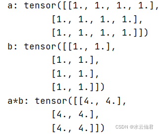
torch.matmul(a,b)——高维矩阵乘积

import torch

a = torch.ones(3,4)
print("a:",a)
b = torch.ones(4,2)
print("b:", b)

print(torch.matmul(a, b))

运行截图

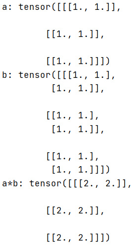
维数相同的高维张量相乘
要求第一维度相同，后两个维度能满足矩阵相乘条件。
A.shape =（b,m,n)；B.shape = (b,n,k)
numpy.matmul(A,B) 结果shape为(b,m,k)

import torch

a = torch.ones(3,1,2)
print(a)
b = torch.ones(3,2,2)
print(b)

print(torch.matmul(a, b))

运行截图

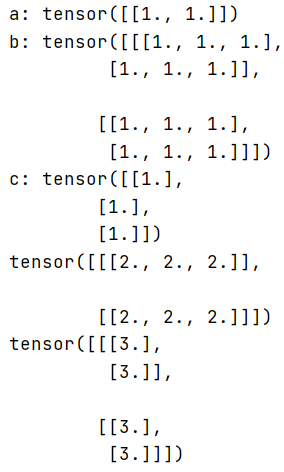
维数不同的高维张量相乘
比如 A.shape =（m,n)； B.shape = (b,n,k)； C.shape=(k,l)
numpy.matmul(A,B) 结果shape为(b,m,k)
numpy.matmul(B,C) 结果shape为(b,n,l)
2D张量要和3D张量的后两个维度满足矩阵相乘条件。

import torch

a = torch.ones(1, 2)
print("a:",a)
b = torch.ones(2, 2, 3)
print("b:",b)
c = torch.ones(3, 1)
print("c:",c)

print("a*b:",torch.matmul(a, b))
print("b*c:",torch.matmul(b, c))

运行截图

微积分

import torch

import numpy as np
from IPython import display
from d2l import torch as d2l


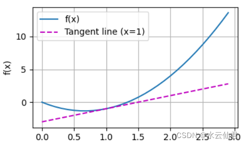
def f(x):
    return 3*x**2-4*x

def numerical_lim(f,x,h):
    return (f(x+h)-f(x))/h

h=0.1
for i in range(5):
    print(f'h={h:.5f},numerical_lim={numerical_lim(f,1,h):.5f}')
    h *= 0.1



def use_svg_display(): #@sava
    '''使用svg格式显示绘图'''
    display.set_matplotlib_formats('svg')

def set_figsize(figsize=(3.5,2.5)): #@save
    '''设置matplotlib的图表大小'''
    use_svg_display()
    d2l.plt.rcParams['figure.figsize'] = figsize

def set_axes(axes,xlabel, ylabel,xlim, ylim, xscale, yscale, legend):
    '''设置matplotlib的轴'''
    axes.set_xlabel(xlabel)
    axes.set_ylabel(ylabel)
    axes.set_xscale(xscale)
    axes.set_yscale(yscale)
    axes.set_xlim(xlim)
    axes.set_ylim(ylim)
    if legend:
        axes.legend(legend)
    axes.grid()

def plot(X,Y=None, xlabel=None,ylabel=None, legend=None, xlim=None,ylim=None,xscale='linear',yscale='linear',
         fmts=('-','m--', 'g-', 'r:'),figsize=(3.5, 2.5),axes=None):
    '''绘制数据点'''
    if legend is None:
        legend = []

    set_figsize(figsize)
    axes = axes if axes else d2l.plt.gca()


    #如果'X'有一个轴，输出True
    def has_one_axis(X):
        return (hasattr(X, 'ndim') and X.ndim == 1 or isinstance(X, list) and not
                hasattr(X[0], '__len__'))
    if has_one_axis(X):
        X=[X]
    if Y is None:
        X,Y = [[]]*len(X),X
    elif has_one_axis(Y):
        Y = [Y]
    if len(X) != len(Y):
        X = X*len(Y)
    axes.cla()
    for x, y, fmt in zip(X, Y, fmts):
        if len(x):
            axes.plot(x,y, fmt)
        else:
            axes.plot(y,fmt)
    set_axes(axes,xlabel,ylabel,xlim, ylim,xscale,yscale,legend)
    d2l.plt.show()

x = np.arange(0,3,0.1)
plot(x,[f(x), 2*x-3], 'x', 'f(x)', legend=['f(x)', 'Tangent line (x=1)'])

自动微分

'''
python3.7
-*- coding: UTF-8 -*-
@Project -> File   ：Code -> __init__.py
@IDE    ：PyCharm
@Author ：YangShouWei
@USER: 296714435
@Date   ：2022/2/19 10:19:49
@LastEditor:
'''

import torch

x = torch.arange(4.0)
print("x:",x)

x.requires_grad_(True) # 等价于x = torch.arange(4.0, requires_grad=True)
print("x.grad:",x.grad) # 默认值是None

y = 2*torch.dot(x,x)
print("y:",y)

# 调⽤反向传播函数来⾃动计算y关于x每个分量的梯度.
y.backward() # 反向传播
x.grad
print("x.grad:",x.grad)

x.grad.zero_()
y = x.sum()
y.backward()
print("x.grad:",x.grad)

# 非标量变量的反向传播
#对⾮标量调⽤`backward`需要传⼊⼀个`gradient`参数，该参数指定微分函数关于`self`的梯度。
# 在我们的例⼦中，我们只想求偏导数的和，所以传递⼀个1的梯度是合适的
x.grad.zero_()
y = x*x

# 等价于y.backward(torch.ones(len(x)))
y.sum().backward()
print("x.grad:",x.grad)

x.grad.zero_() # 梯度置0
y = x*x
u = y.detach()
z = u*x
z.sum().backward()
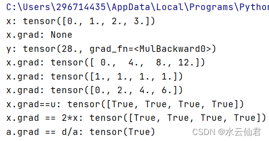
print("x.grad==u:",x.grad==u)

# 由于记录了y的计算结果，我们可以随后在y上调⽤反向传播，得到y=x*x关于的x的导数，即2*x。
x.grad.zero_()
y.sum().backward()
print("x.grad == 2*x:",x.grad == 2*x)

# Python 控制流的梯度计算
def f(a):
    b = a*2
    while b.norm() < 1000:
        b=b*2
    if b.sum() > 0:
        c = b
    else:
        c = 100*b
    return c

# 计算梯度
a = torch.randn(size=(), requires_grad=True)
d = f(a)
d.backward()

print("a.grad == d/a:",a.grad == d/a)

运行截图

概率

基本概率论

'''
python3.7
-*- coding: UTF-8 -*-
@Project -> File   ：Code -> probability
@IDE    ：PyCharm
@Author ：YangShouWei
@USER: 296714435
@Date   ：2022/2/19 14:46:22
@LastEditor:
'''

import torch
from torch.distributions import multinomial
from d2l import torch as d2l

# 为了抽取⼀个样本，即掷骰⼦，我们只需传⼊⼀个概率向量。
# 输出是另⼀个相同⻓度的向量：它在索引i处的值是采样结果中i出现的次数。

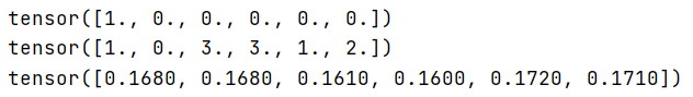
fair_prob = torch.ones([6]) / 6 # 表示骰子的六个面被掷到的概率都是1/6
print(multinomial.Multinomial(1,fair_prob).sample()) # 相当于掷骰子一次，掷到哪个数字，对应位置就显示1，

print(multinomial.Multinomial(10,fair_prob).sample()) # 相当于掷骰子10次，打印的结果是每个面被掷到的次数

counts = multinomial.Multinomial(1000,fair_prob).sample()
print(counts/1000) # 相对频率作为估计值


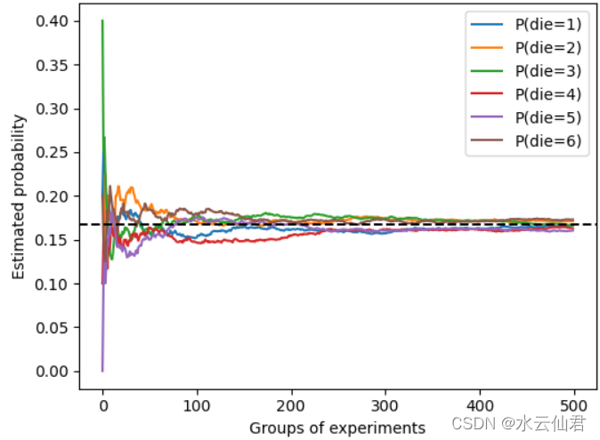
# 进行500组实验，每组抽取10个样本
counts = multinomial.Multinomial(10,fair_prob).sample((500,))
cum_counts = counts.cumsum(dim=0)
estimates = cum_counts / cum_counts.sum(dim=1, keepdims=True)

d2l.set_figsize((6, 4.5))
for i in range(6):
    d2l.plt.plot(estimates[:, i].numpy(),
                 label=("P(die="+str(i+1)+")"))
d2l.plt.axhline(y=0.167,color='black',linestyle='dashed')
d2l.plt.gca().set_xlabel("Groups of experiments")
d2l.plt.gca().set_ylabel("Estimated probability")
d2l.plt.legend();
d2l.plt.show()

运行截图

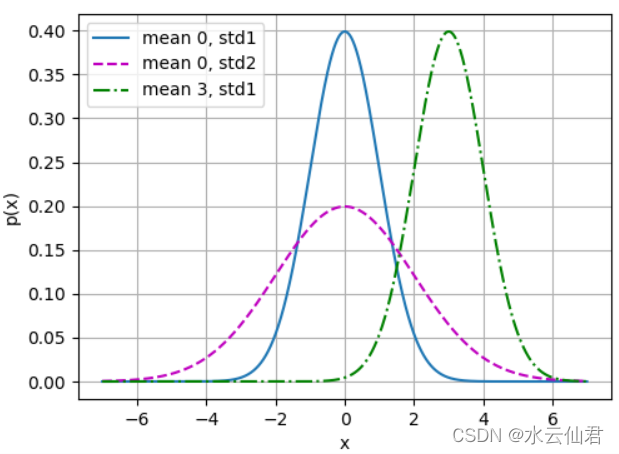
正太分布与平方损失

import math
import numpy as np
from d2l import torch as d2l

def normal(x, mu, sigma):
    """
    计算正太分布
    """
    p = 1/math.sqrt(2 * math.pi * sigma**2)
    return p*np.exp(-0.5/sigma**2 * (x-mu)**2)

if __name__ == '__main__':
    #使用numpy进行可视化
    x = np.arange(-7, 7, 0.01)

    #均值和标准差对
    params = [(0, 1),(0, 2),(3,1)]
    d2l.plot(x, [normal(x, mu, sigma) for mu, sigma in params], xlabel='x',
             ylabel='p(x)', figsize=(5.5, 4.0),
             legend=[f'mean {mu}, std{sigma}'for mu, sigma in params])
    d2l.plt.show()

运行截图

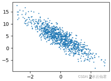
生成数据集

from d2l import torch as d2l
import torch

def synthetix_data(w,b, num_examples):
    """⽣成y = Xw + b + 噪声。"""

    """返回一个张量，包含从给定参数means,std的离散正态分布中抽取随机数。 均值means是一个张量，包含每个输出元素相关的正态分布的均值。
    std是一个张量，包含每个输出元素相关的正态分布的标准差。 均值和标准差的形状不须匹配，但每个张量的元素个数须相同。"""
    X = torch.normal(0, 1, (num_examples, len(w)))
    # print(X)
    y = torch.matmul(X, w) +b # 张量乘法
    # print(y)
    y += torch.normal(0, 0.01, y.shape)
    return X, y.reshape((-1, 1))


true_w = torch.tensor([2, -3.4])
true_b = 4.2
features, labels = synthetix_data(true_w, true_b, 1000)

d2l.set_figsize()
d2l.plt.scatter(features[:,(1)].detach().numpy(), labels.detach().numpy(),1)
d2l.plt.show()

数据分布图