


YOLOv3模型训练
前面我们已经讲解了模型的搭建和数据类,现在可以来正式训练模型了。
1 迁移学习
(1)两种权重文件
我们基本不会去从0开始训练模型,而是从官网把已经训练好的模型导入,即迁移学习。
在yolo3_from_scratch中新建一个名为weights的文件夹,将权重文件放入,权重文件有两种,一种是整个模型的参数文件,另一种是backbone的参数文件。将两种权重文件加入后,那么项目结构将如下图所示:

(2)导入权重方法
在models.py的Darknet类中,增加一个导入权重的方法,其代码如下:
    def load_darknet_weights(self, weights_path):
        """Parses and loads the weights stored in 'weights_path'"""

        # Open the weights file
        with open(weights_path, "rb") as f:         # 以二进制方式打开文件
            header = np.fromfile(f, dtype=np.int32, count=5)  # First five are header values
            self.header_info = header  # Needed to write header when saving weights
            self.seen = header[3]  # number of images seen during training
            weights = np.fromfile(f, dtype=np.float32)  # The rest are weights 将二进制文件转化为numpy数组

        # Establish cutoff for loading backbone weights
        # 如果只想导入backbone,那么就需要设定一个cutoff变量,用于停止导入数据
        cutoff = None
        if "darknet53.conv.74" in weights_path:
            cutoff = 75

        ptr = 0     # 这就类似于一个指针,确定每次导入数据从哪个位置开始
        for i, (module_def, module) in enumerate(zip(self.module_defs, self.module_list)):
            if i == cutoff:
                # 当i为75时,说明backbone部分的迁移学习结束了,此时退出循环
                break
            if module_def["type"] == "convolutional":
                conv_layer = module[0]
                if module_def["batch_normalize"]:
                    # Load BN bias, weights, running mean and running variance
                    bn_layer = module[1]
                    num_b = bn_layer.bias.numel()  # Number of biases
                    # Bias
                    bn_b = torch.from_numpy(weights[ptr : ptr + num_b]).view_as(bn_layer.bias)
                    bn_layer.bias.data.copy_(bn_b)
                    ptr += num_b
                    # Weight
                    bn_w = torch.from_numpy(weights[ptr : ptr + num_b]).view_as(bn_layer.weight)
                    bn_layer.weight.data.copy_(bn_w)
                    ptr += num_b
                    # Running Mean
                    bn_rm = torch.from_numpy(weights[ptr : ptr + num_b]).view_as(bn_layer.running_mean)
                    bn_layer.running_mean.data.copy_(bn_rm)
                    ptr += num_b
                    # Running Var
                    bn_rv = torch.from_numpy(weights[ptr : ptr + num_b]).view_as(bn_layer.running_var)
                    bn_layer.running_var.data.copy_(bn_rv)
                    ptr += num_b
                else:
                    # Load conv. bias
                    num_b = conv_layer.bias.numel()
                    conv_b = torch.from_numpy(weights[ptr : ptr + num_b]).view_as(conv_layer.bias)
                    conv_layer.bias.data.copy_(conv_b)
                    ptr += num_b
                # Load conv. weights
                num_w = conv_layer.weight.numel()
                conv_w = torch.from_numpy(weights[ptr : ptr + num_w]).view_as(conv_layer.weight)
                conv_layer.weight.data.copy_(conv_w)
                ptr += num_w
现在可以在最后添加一段测试代码:
if __name__ == '__main__':
    """测试两种迁移学习"""

    test_input = torch.rand((2, 3, 416, 416))

    # 建立模型并导入配置文件
    file_path = r"config/yolov3.cfg"
    model = Darknet(file_path)

    # 第一种:导入整个模型的参数文件
    model.load_darknet_weights(r"weights/yolov3.weights")
    pred1 = model(test_input)
    print(pred1.shape)
    print(pred1)

	# 第二种:导入backbone的参数文件
    model.load_darknet_weights(r"weights/darknet53.conv.74")
    pred2 = model(test_input)
    print('-'*50)
    print(pred2.shape)
    print(pred2)
输出


(3)保存模型的方法
因为导入的权重文件并不是.pth文件,而是.weight文件,为了能协调,我们保存模型参数的时候,也将其保存为.weight文件,当某次训练终端,下次继续训练的时候,可以像最开始一样使用model.load_darknet_weights方法调用上次保存的参数,可以从上个断点开始训练。
    def save_darknet_weights(self, path, cutoff=-1):
        """
            @:param path    - path of the new weights file
            @:param cutoff  - save layers between 0 and cutoff (cutoff = -1 -> all are saved)
        """
        fp = open(path, "wb")
        self.header_info[3] = self.seen
        self.header_info.tofile(fp)

        # Iterate through layers
        for i, (module_def, module) in enumerate(zip(self.module_defs[:cutoff], self.module_list[:cutoff])):
            if module_def["type"] == "convolutional":
                conv_layer = module[0]
                # If batch norm, load bn first
                if module_def["batch_normalize"]:
                    bn_layer = module[1]
                    bn_layer.bias.data.cpu().numpy().tofile(fp)
                    bn_layer.weight.data.cpu().numpy().tofile(fp)
                    bn_layer.running_mean.data.cpu().numpy().tofile(fp)
                    bn_layer.running_var.data.cpu().numpy().tofile(fp)
                # Load conv bias
                else:
                    conv_layer.bias.data.cpu().numpy().tofile(fp)
                # Load conv weights
                conv_layer.weight.data.cpu().numpy().tofile(fp)

        fp.close()
2 标签转化函数
之前在介绍YOLOLayer时,计算损失函数前,有个函数是build_targets,当时因为还没有讲数据集,所以就没有展开来讲,现在可以具体介绍了。
build_targets是标签转化函数,原来的targets标签,很难直接用来计算损失函数,所以这里必须将其转化,它的基本思想是建立若干个0张量,然后根据targets的信息,给这些0张量的对应位置赋值,未得到赋值的,说明该位置无目标。具体代码如下(在utils/utils.py中):
def build_targets(pred_boxes, pred_cls, target, anchors, ignore_thres):
    """
    这是根据标签和
    :param pred_boxes: 维度为(batch_size, 3, grid_size, grid_size, 4),即预测的目标框信息
    :param pred_cls: 维度为(batch_size, 3, grid_size, grid_size, 80),即预测的目标类别编号
    :param target: 维度为(num_objects, 6),其中num_objects是该batch的所有图片的目标总数
                即后面5列分别是bbox的分类索引,和位置以及高宽(已归一化)
    :param anchors: 维度是(3,2),调用本函数的YOLO模块对应的anchors,必须是缩放后的anchors,
    :param ignore_thres: iou阈值
    :return:
    """

    ByteTensor = torch.cuda.ByteTensor if pred_boxes.is_cuda else torch.ByteTensor
    FloatTensor = torch.cuda.FloatTensor if pred_boxes.is_cuda else torch.FloatTensor

    nB = pred_boxes.size(0) # batch_size 4
    nA = pred_boxes.size(1) # 每个格子对应了多少个anchor
    nC = pred_cls.size(-1)  # 类别的数量
    nG = pred_boxes.size(2) # gridsize

    # Output tensors
    obj_mask = ByteTensor(nB, nA, nG, nG).fill_(0)  # obj,anchor包含物体, 即为1,默认为0 考虑前景
    noobj_mask = ByteTensor(nB, nA, nG, nG).fill_(1) # noobj, anchor不包含物体, 则为1,默认为1 考虑背景
    class_mask = FloatTensor(nB, nA, nG, nG).fill_(0) # 类别掩膜,类别预测正确即为1,默认全为0
    iou_scores = FloatTensor(nB, nA, nG, nG).fill_(0) # 预测框与真实框的iou得分

    tx = FloatTensor(nB, nA, nG, nG).fill_(0)       # 真实框相对于网格的位置
    ty = FloatTensor(nB, nA, nG, nG).fill_(0)
    tw = FloatTensor(nB, nA, nG, nG).fill_(0)
    th = FloatTensor(nB, nA, nG, nG).fill_(0)
    tcls = FloatTensor(nB, nA, nG, nG, nC).fill_(0)

    # Convert to position relative to box
    target_boxes = target[:, 2:6] * nG # target中的xywh都是0-1的,可以得到其在当前gridsize上的xywh
    gxy = target_boxes[:, :2]           # 维度为(num_objects, 2)
    gwh = target_boxes[:, 2:]           # 维度为(num_objects, 2)

    # Get anchors with best iou
    ious = torch.stack([bbox_wh_iou(anchor, gwh) for anchor in anchors])
    # 计算每一种规格的anchor跟每个标签上的框的IOU得分(假设边框中心重合)
    # 每次调用bbox_wh_iou(anchor, gwh)返回的结果是一个一维数组,维度为(num_objects, )
    # 上面这条命令,先用一个列表推导式生成一个列表,列表中的每个元素都是一维数组
    # 经过torch.stack堆叠之后,得到一个维度为(3, num_objects)的张量
    # 即ious的维度为(3, num_objects)

	# print (ious.shape)
    best_ious, best_n = ious.max(0) # 得到其最高分以及哪种规格框和当前目标最相似
    # best_ious是每一列的最大值
    # best_n是最大值所在的索引(行号),即GroundTruth(下面简称GT)的形状和哪个anchor匹配
这里出现了bbox_wh_iou,它是将两个box的中心放到一块,然后计算交并比,目的是根据交并比,为每个真实框选择最相似的anchor,在build_targets后面加入下面的函数:
def bbox_wh_iou(wh1, wh2):
    """
    因为特征层中每个
    :param wh1: box1的宽高,维度为(2, ),即一维数组
    :param wh2: box2的宽高,维度为(num_objects, 2),第一列是宽,第二列是高
    :return: 返回交并比,维度为(num_objects, ),即一维数组
    """
    wh2 = wh2.t()
    # 转置之后,wh2的维度为(2, num_objects),
    # 这样就能保证wh2[0]是宽, wh2[1]是高

    w1, h1 = wh1[0], wh1[1]
    w2, h2 = wh2[0], wh2[1]
    inter_area = torch.min(w1, w2) * torch.min(h1, h2)      # 计算交集
    union_area = (w1 * h1 + 1e-16) + w2 * h2 - inter_area   # 计算并集

    # 返回交并比
    return inter_area / union_area
回到build_targets函数中,前面已经为每个真实框找到了最接近的anchor,现在可以根据targets,找到哪些图片存在目标,目标又存在于图片的哪个网格中,也就是说,可以给iou_scores, class_mask, obj_mask, noobj_mask, tx, ty, tw, th, tcls, tconf
的对应位置赋值
    # Separate target values
    b, target_labels = target[:, :2].long().t()
    # b表示真实框对应的图片在batch中的索引(即由索引构成的数组),
    # 比如索引为1的图片中有两个目标,那么1在数组b中将出现2次
    # target_labels则为类别索引

    gx, gy = gxy.t()        # gxy转置之维度为(2, num_objects),gx和gy的维度都是(num_objects, )
    gw, gh = gwh.t()        # gwh转置之维度为(2, num_objects),gw和gh的维度都是(num_objects, )
    gi, gj = gxy.long().t() # 位置信息,向下取整了

    # Set masks
    obj_mask[b, best_n, gj, gi] = 1     # 为每个网格选择最接近标签值的anchor,只有与标签最接近的anchor才赋1
    noobj_mask[b, best_n, gj, gi] = 0   # 与obj_mask相反
    # b,best_n,gj, gi,他们都是维度为(num_objects, )的数组
    # b为目标的图片索引,best_n为目标对应的anchor的索引,他们都是维度为(num_objects, )的数组
    # gj为目标在特征图中对应的列号,gi为行号

    # Set noobj mask to zero where iou exceeds ignore threshold
    for i, anchor_ious in enumerate(ious.t()): # IOU超过了指定的阈值就相当于有物体了
        # ious.t()的维度为(num_objects, 3)
        # anchor_ious的维度为(3, )
        noobj_mask[b[i], anchor_ious > ignore_thres, gj[i], gi[i]] = 0  # 布尔索引

    # TODO 为何不对obj_mask做类似的处理,比如把iou低于阈值的设为0

    # Coordinates
    tx[b, best_n, gj, gi] = gx - gx.floor() # 根据真实框所在位置,得到其相当于网络的位置
    ty[b, best_n, gj, gi] = gy - gy.floor() #

    # Width and height
    tw[b, best_n, gj, gi] = torch.log(gw / anchors[best_n][:, 0] + 1e-16)
    th[b, best_n, gj, gi] = torch.log(gh / anchors[best_n][:, 1] + 1e-16)

    # One-hot encoding of label
    tcls[b, best_n, gj, gi, target_labels] = 1 # 将真实框的标签转换为one-hot编码形式
    # tcls本来全部是0,现在根据类别信息在特定的位置赋1

    # 对类别预测正确的目标,在class_mask的对应位置赋1
    class_mask[b, best_n, gj, gi] = (pred_cls[b, best_n, gj, gi].argmax(-1) == target_labels).float()

    # 求真实框与对应位置的预测框的iou值
    iou_scores[b, best_n, gj, gi] = bbox_iou(pred_boxes[b, best_n, gj, gi], target_boxes, x1y1x2y2=False)

    tconf = obj_mask.float() # 真实框的置信度,也就是1

    # iou_scores和class_mask是根据真实框与对应位置的预测框相比较得到的
    # obj_mask, noobj_mask, tx, ty, tw, th, tcls, tconf均来源于标签(真实框)
    return iou_scores, class_mask, obj_mask, noobj_mask, tx, ty, tw, th, tcls, tconf
上面还出现了bbox_iou函数,这是用来计算两个box的交并比,和前面的bbox_wh_iou不一样的是,bbox_iou没有把两个目标框的中心点放到一块,其代码如下(放到utils/utils.py中):
def bbox_iou(box1, box2, x1y1x2y2=True):
    """
    Returns the IoU of two bounding boxes
    :param box1:维度为(num_objects, 4)
    :param box2:维度为(num_objects, 4)
    :param x1y1x2y2: 表示输入的目标框是否为上下角点坐标
    :return:
    """

    # 获得边框左上角点和右下角点的坐标
    if not x1y1x2y2:
        # Transform from center and width to exact coordinates
        b1_x1, b1_x2 = box1[:, 0] - box1[:, 2] / 2, box1[:, 0] + box1[:, 2] / 2
        b1_y1, b1_y2 = box1[:, 1] - box1[:, 3] / 2, box1[:, 1] + box1[:, 3] / 2
        b2_x1, b2_x2 = box2[:, 0] - box2[:, 2] / 2, box2[:, 0] + box2[:, 2] / 2
        b2_y1, b2_y2 = box2[:, 1] - box2[:, 3] / 2, box2[:, 1] + box2[:, 3] / 2
    else:
        # Get the coordinates of bounding boxes
        b1_x1, b1_y1, b1_x2, b1_y2 = box1[:, 0], box1[:, 1], box1[:, 2], box1[:, 3]
        b2_x1, b2_y1, b2_x2, b2_y2 = box2[:, 0], box2[:, 1], box2[:, 2], box2[:, 3]

    # get the corrdinates of the intersection rectangle
    # 计算真实框与预测框的交集矩形的左上角点和右下角点的坐标
    inter_rect_x1 = torch.max(b1_x1, b2_x1)
    inter_rect_y1 = torch.max(b1_y1, b2_y1)
    inter_rect_x2 = torch.min(b1_x2, b2_x2)
    inter_rect_y2 = torch.min(b1_y2, b2_y2)

    # Intersection area交集面积
    inter_area = torch.clamp(inter_rect_x2 - inter_rect_x1 + 1, min=0) * torch.clamp(
        inter_rect_y2 - inter_rect_y1 + 1, min=0
    )
    # torch.clamp是上下限控制函数,这里使用这个函数,是因为真实框与目标框可能不存在交集
    # 那么inter_rect_x2-inter_rect_x1+1 或者 inter_rect_y2 - inter_rect_y1+1 就是负的
    # TODO 这里inter_rect_x2-inter_rect_x1+1,后面为什么要加1,有评论说是计算交集像素值
    # TODO 这里inter_rect_x2是相对于特征层的位置,这里不再深究,就先把问题放在这里

    # Union Area
    b1_area = (b1_x2 - b1_x1 + 1) * (b1_y2 - b1_y1 + 1)     # box1的面积
    b2_area = (b2_x2 - b2_x1 + 1) * (b2_y2 - b2_y1 + 1)     # box2的面积

    iou = inter_area / (b1_area + b2_area - inter_area + 1e-16)     # 计算交并比

    return iou
可以写一个测试脚本(名为build_targets_test.py),测试一下build_targets函数,代码如下:
# coding=utf-8
import torch
from utils.datasets import ListDataset
from models import Darknet

import warnings
warnings.filterwarnings("ignore")   # 过滤掉警告

train_path = r"F:\thesis\yolo3_from_scratch\data\coco128\train_path.txt"
dataset = ListDataset(train_path, augment=True, multiscale=True)
dataloader = torch.utils.data.DataLoader(
    dataset,
    batch_size=2,
    shuffle=False,              # 这边不能打乱
    collate_fn=dataset.collate_fn,  #
)

model = Darknet(r"config/yolov3.cfg")
model.load_darknet_weights(r"weights/yolov3.weights")

model.eval()
for batch_i, (_, imgs, targets) in enumerate(dataloader):
    loss, outputs = model(imgs, targets)
    print(loss.shape)       # 从结果可以看到,loss是零维数组
    print(loss)
    print(outputs.shape)
    break
输出:
torch.Size([])
tensor(30.5892, grad_fn=<AddBackward0>)
torch.Size([2, 16128, 85])
3 模型训练
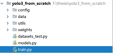
在yolo3_from_scratch中新建一个名为train.py的脚本,建立后,项目结构如下:
在train.py中,我们先先将需要的模块导入
from __future__ import division

from models import *
from utils.logger import *
from utils.utils import *
from utils.datasets import *
from utils.parse_config import *
from test import evaluate

import warnings
warnings.filterwarnings("ignore")   # 过滤掉警告

from terminaltables import AsciiTable

import os
import sys
import time
import datetime
import argparse

import torch
from torch.utils.data import DataLoader
from torchvision import datasets
from torchvision import transforms
from torch.autograd import Variable
import torch.optim as optim
我们使用命令行输入的方式输出超参数,那么必须有argparse.ArgumentParser()对象,然后往里添加参数
if __name__ == "__main__":
    parser = argparse.ArgumentParser()
    parser.add_argument("--epochs", type=int, default=100, help="number of epochs")
    parser.add_argument("--batch_size", type=int, default=4, help="size of each image batch")
    parser.add_argument("--gradient_accumulations", type=int, default=2, help="number of gradient accums before step")
    parser.add_argument("--model_def", type=str, default="config/yolov3.cfg", help="path to model definition file")
    parser.add_argument("--data_config", type=str, default="config/coco.data", help="path to data config file")
    parser.add_argument("--pretrained_weights", type=str, help="if specified starts from checkpoint model")
    parser.add_argument("--n_cpu", type=int, default=0, help="number of cpu threads to use during batch generation")
    parser.add_argument("--img_size", type=int, default=416, help="size of each image dimension")
    parser.add_argument("--checkpoint_interval", type=int, default=1, help="interval between saving model weights")
    parser.add_argument("--evaluation_interval", type=int, default=1, help="interval evaluations on validation set")
    parser.add_argument("--compute_map", default=False, help="if True computes mAP every tenth batch")
    parser.add_argument("--multiscale_training", default=True, help="allow for multi-scale training")
    opt = parser.parse_args()
    print(opt)
我们来逐个介绍一下上面参数的具体含义:
–epochs是数据集遍历次数;
–batch_size是每个batch的样本个数;
–gradient_accumulations 梯度累计,我们这里并非每获得一次梯度就下降一次,而是积攒若干个batch的梯度后,再下降一次,多少次梯度下降一次,即由参数 gradient_accumulations 决定;
–model_def 模型的配置文件地址
–data_config 数据配置文件的地址
–pretrained_weights 预训练权重文件地址
–n_cpu 在生成batch的时候,指定核数
–img_size 指定图片的输入尺寸,这里必须是32的倍数
–checkpoint_interval 每遍历多少次(数据)保存一次模型
–evaluation_interval 每遍历多少次(数据)评估一次模型
–compute_map 是否每10个batch计算一次mAP
–multiscale_training 是否使用多尺度训练(在utils/datasets.py的数据集类ListDataset的collate_fn函数中,每10个batch随机改变一次输入图片的尺寸)
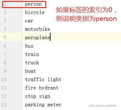
这里有个数据配置 data_config,这来需要讲解一下。在上一节数据的组织的时候,我们说过,边框中的类别由首列数字决定,首列数字到底代表了什么呢?所以必须将数字与具体的类名给对应起来。将coco.names复制到yolo3_from_scratch/data下,它每一行代表一个类别,比如第一行是person,而类别索引是从0开始的,如果某个类别索引为0,则从coco.names中要到最开始的那一行(person),即为该目标的类别。coco.names的部分内容如下:
此时项目结构为:

有了coco.names的文件,还要建立一个解析它的方法,在utils/utils中,加入下面的函数
def load_classes(path):
    """
    Loads class labels at 'path'
    """
    fp = open(path, "r")
    names = fp.read().split("\n")[:-1]
    fp.close()
    return names
现在要建立一个文件,将train_path.txt、test_path.txt以及coco.names三个文件统合起来,在yolo3_from_srcatch/config下建立一个名为coco.data的文件,其内容如下:
classes= 80
train=data/coco/train_path.txt
valid=data/coco/test_path.txt
names=data/coco.names
此时项目结构为:

现在要建立一个解析coco.data的函数,在utils/parse_config.py中新建一个名为parse_data_config函数其代码如下:
def parse_data_config(path):
    """Parses the data configuration file,返回一个字典,该字典为数据配置文件的信息"""
    options = dict()
    options['gpus'] = '0,1,2,3'     # TODO 这里为何要加上GPU的信息
    options['num_workers'] = '10'   # TODO 这里为何要加上num_workers?
    with open(path, 'r') as fp:
        lines = fp.readlines()
    for line in lines:  # 一行一行的地解析配置文件
        line = line.strip()
        if line == '' or line.startswith('#'):
            continue
        key, value = line.split('=')
        options[key.strip()] = value.strip()
    return options
让我们回到train.py中,接下来是解析配置文件并建立模型
    # 确定使用GPU还是CPU
    device = torch.device("cuda" if torch.cuda.is_available() else "cpu")

    # 解析数据配置文件
    data_config = parse_data_config(opt.data_config)  # 解析关于数据的配置文件,即config/coco.data
    train_path = data_config["train"]             # 获取训练集样本路径地址
    valid_path = data_config["valid"]               # 获取验证集样本路径地址
    class_names = load_classes(data_config["names"])  # 获得类别名

    # 建立模型并初始化
    model = Darknet(opt.model_def).to(device)  # 导入配置文件建立模型,并放入GPU中
    model.apply(weights_init_normal)  # 权重初始化,weights_init_normal是utils/utils.py中的方法
    # model.apply(weights_init_normal)表示对model中的每个参数都使用weights_init_normal方法进行初始化
这里有个权重初始化方法,我们这里其实完全不用初始化,但对模型的作者来说,他必须从零开始训练,所以从作者的角度来说,必须要有初始化方法。可以在utils/utils.py中把这个方法添加上去,代码如下:
def weights_init_normal(m):
    classname = m.__class__.__name__    # 获取类名
    if classname.find("Conv") != -1:
        torch.nn.init.normal_(m.weight.data, 0.0, 0.02)
    elif classname.find("BatchNorm2d") != -1:
        torch.nn.init.normal_(m.weight.data, 1.0, 0.02)
        torch.nn.init.constant_(m.bias.data, 0.0)
回到train.py当中,接下来是迁移学习,代码如下:
    if opt.pretrained_weights:
        if opt.pretrained_weights.endswith(".pth"):  # 有可能导入的是整个模型
            model.load_state_dict(torch.load(opt.pretrained_weights))
        else:  # 也有可能导入的是模型的权重
            model.load_darknet_weights(opt.pretrained_weights)
接下来是实例化一个数据导入器,代码如下:
    # Get dataloader
    dataset = ListDataset(train_path, augment=True, multiscale=opt.multiscale_training)
    dataloader = torch.utils.data.DataLoader(
        dataset,
        batch_size=opt.batch_size,
        shuffle=True,
        num_workers=opt.n_cpu,
        pin_memory=True,  # 是否在返回前,将数据复制到显存中
        collate_fn=dataset.collate_fn,
    )
然后是优化器,这里我们使用Adam优化方法
optimizer = torch.optim.Adam(model.parameters()) # 指定优化器
接下来是模型的评价指标
    metrics = [
        "grid_size",
        "loss",
        "x",
        "y",
        "w",
        "h",
        "conf",
        "cls",
        "cls_acc",
        "recall50",
        "recall75",
        "precision",
        "conf_obj",
        "conf_noobj",
    ]
还记得YOLOLayer模块中,有个self.metrics吗,这里的metrics和YOLOLayer模块中的self.metrics是一样的,仅仅是顺序稍微有点不一致。
接下来就是迭代了,写一个for循环,在for循环里面,把model设定为训练模式:
    for epoch in range(opt.epochs):
        model.train()               # 切换到训练模式
        start_time = time.time()    # 记录时间
再往里嵌套一个for循环
        for batch_i, (_, imgs, targets) in enumerate(dataloader):
            batches_done = len(dataloader) * epoch + batch_i
            # batches_done表示第几次迭代

            # 图片和标签做成变量
            imgs = Variable(imgs.to(device))
            targets = Variable(targets.to(device), requires_grad=False)

            loss, outputs = model(imgs, targets)	# 前向传播
            loss.backward()                         # 根据损失函数更新梯度


            if batches_done % opt.gradient_accumulations:
                # Accumulates gradient before each step
                # 这里并非每次得到梯度就更新,而是累积若干次梯度才进行更新
                optimizer.step()
                optimizer.zero_grad()   # 梯度信息清零

			# 迭代进度
			log_str = "\n---- [Epoch %d/%d, Batch %d/%d] ----\n" % (epoch, opt.epochs, batch_i, len(dataloader))
将当前batch的统计指标写入log对象
            metric_table = [["Metrics", *[f"YOLO Layer {i}" for i in range(len(model.yolo_layers))]]]
            # 列表当中嵌套列表,上面的命令执行后,结果如下:
            # [["Metrics", "YOLO Layer 0", "YOLO Layer 1", "YOLO Layer 2"]]

            # Log metrics at each YOLO layer
            for i, metric in enumerate(metrics):
                formats = {m: "%.6f" for m in metrics}  # 字典生成式
                formats["grid_size"] = "%2d"
                formats["cls_acc"] = "%.2f%%"		# 第一个%表示和字符串相连,后面两个%用来输出%,其中一个用来转义

                row_metrics = [formats[metric] % yolo.metrics.get(metric, 0) for yolo in model.yolo_layers]
                # metric是metrics中的元素,即一个字符串,formats[metric]是根据键从字典中取值
                # yolo.metrics.get(metric, 0),这里调用了字典的get方法,根据关键字获取值,如果没有这个关键字,则返回0
                # 由于formats[metric]是"%.6f"(除了formats["grid_size"]和formats["cls_acc"])
                # formats[metric] % yolo.metrics.get(metric, 0)相当于"%.6f"% number,即按格式拼接字符串

                metric_table += [[metric, *row_metrics]]
                # 第一轮循环时,metric为grid_size,row_metrics的结果为['16','32','64']
                # 上条命令执行之后,metric_table为
                #  [['Metrics', 'YOLO Layer 0', 'YOLO Layer 1', 'YOLO Layer 2'],
                #   ['grid_size', '16', '32', '64']]

                # Tensorboard logging
                tensorboard_log = []
                for j, yolo in enumerate(model.yolo_layers):
                    for name, metric in yolo.metrics.items():
                        if name != "grid_size":
                            tensorboard_log += [(f"{name}_{j+1}", metric)]  # TODO j为何要加1,因为j是从0开始计数
                            # 第一轮循环后,tensorboard_log为[('loss_1', 73.77989196777344)]
                            # 上面实际上是将每个YOLO头的评价指标写入tensorboard_log中

                # 因为tensorboard_log = [] 在for batch_i, (_, imgs, targets) 的循环内部
                # 因此相当于每一轮循环,tensorboard_log都指向了一个空列表
                tensorboard_log += [("loss", loss.item())]
                # TODO 同一个batch_i中,每次循环获得的tensorboard_log都是一样的,
                # TODO 那么为何每次都要重新计算呢,难道就是为了和batches_done共同使用吗?

                # 将tensorboard_log写入log对象
                logger.list_of_scalars_summary(tensorboard_log, batches_done)
现在可以跳出for i, metric in enumerate(metrics):循环了,为了显示当前模型的评价指标,我们把metric_table做成二进制表格,然后计算训练还需要多少时间,将需要的信息转成字符串拼接起来并输出,代码如下:
            log_str += AsciiTable(metric_table).table
            log_str += f"\nTotal loss {loss.item()}"

            # Determine approximate time left for epoch

            # 计算当前epoch还剩下多少个batch未迭代
            epoch_batches_left = len(dataloader) - (batch_i + 1)

            # 计算还需要多少时间才能训练完
            time_left = datetime.timedelta(seconds=epoch_batches_left * (time.time() - start_time) / (batch_i + 1))
            log_str += f"\n---- ETA {time_left}"
            model.seen += imgs.size(0)  # 表示模型已经看过多少张图片,其实这个属性的作用不大
            print(log_str)
            """输出的是下面这一大串:
            ---- [Epoch 0/100, Batch 0/59] ----
            +------------+--------------+--------------+--------------+
            | Metrics    | YOLO Layer 0 | YOLO Layer 1 | YOLO Layer 2 |
            +------------+--------------+--------------+--------------+
            | grid_size  | 16           | 32           | 64           |
            | loss       | 68.630249    | 73.688156    | 73.450012    |
            | x          | 0.098111     | 0.087221     | 0.065444     |
            | y          | 0.203116     | 0.053111     | 0.078177     |
            | w          | 1.446948     | 1.016232     | 1.415377     |
            | h          | 3.089972     | 1.110960     | 2.104409     |
            | conf       | 63.065159    | 70.704948    | 69.075424    |
            | cls        | 0.726945     | 0.715680     | 0.711185     |
            | cls_acc    | 22.22%       | 0.00%        | 0.00%        |
            | recall50   | 0.000000     | 0.000000     | 0.000000     |
            | recall75   | 0.000000     | 0.000000     | 0.000000     |
            | precision  | 0.000000     | 0.000000     | 0.000000     |
            | conf_obj   | 0.402709     | 0.552602     | 0.548954     |
            | conf_noobj | 0.454951     | 0.496319     | 0.492412     |
            +------------+--------------+--------------+--------------+
            Total loss 215.76841735839844
            ---- ETA 1:19:17.722132"""
train.py的程序并未结束,后面会继续讲,这里我们先切换到模型的评价
4.模型评价
(1)mAP的计算原理
目标检测模型最重要的评价指标,是mAP,我们先来说一下mAP的计算过程。
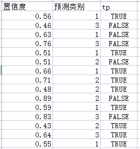
假设一个batch的所有图片经过NMS(假设NMS时,置信度阈值为0.4,)之后,还剩下15个预测框,它们的信息如下:

现在再计算每个预测框与所在图片的GT的iou值。比如计算id为0的预测框的iou,假设该图片中所有类别加起来有5个GT,那么就计算这个预测框与这5个GT的iou,即先不管类别是否和预测框一致,先算了再说,然后取这5个iou的最大值作为“与GT的iou”(严格地说,计算“与GT的iou”时,应该计算预测框与同类别GT的iou最大值,但从程序的实现来看,计算的并不是同类,而是计算与所有类别的GT的最大值,因此这里是有问题的)。结果如下:

接下来要筛选合格的边框,这里新增一列tp,设iou_thres=0.5,若iou>iou_thres,那么tp=True,否则tp=False,新增tp之后,结果为:

上面表格中的tp、置信度和预测类别,就是get_batch_statistics函数(后面的程序会介绍)的返回结果。
回到evaluate函数,将当前batch的get_batch_statistics函数的返回值加入到列表sample_metrics中,然后通过np.concatenate函数将不同batch的tp、置信度和预测类别三列进行拼接,得到整个验证集上的tp、置信度和预测类别。
下面介绍ap_per_class函数,为了便于讲解,我们假设这里只有一个batch,即认为上面的表格,就是整个验证集上所有的预测框。
由于只有三列被输入到了这个函数中,所以在刚进入ap_per_class函数时,整个验证集的所有预测框是这样的:
接下来按照置信度对预测框进行从大到小排序,结果如下:
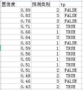
假设GT也有编号为1、2、3共三个类别,接下来就是逐个类别计算AP(注意,AP的计算是将整个验证集中所有图片的所有合格预测框归并起来,然后逐个类别地计算,而不是对每张图片的每个类别单独计算AP)。
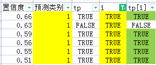
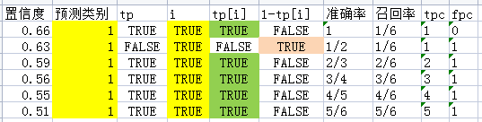
先计算类别1的AP。这里新增一列i,若预测类别为1,则i为True,否则i为False,新增i之后,结果如下(将类别为1的预测框用黄色标出):

在后面新增一列tp[i](对tp进行布尔索引,也就是i为True的行,获得的行数必然小于tp的行数),新增之后为:
在后面新增一列1-tp[i],新增之后为:
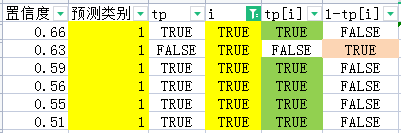
tp[i]为True的预测框其实就是TP(绿色部分所在行),因为这些预测框与GT的iou的最大值超过了iou_thres,因此对于类别1来说,它们本来就是正样本,而且被成功预测出来了,即True Positive。
1-tp[i]为True的预测框其实就是FP(粉色部分所在行),因为它们与GT的iou最大值小于iou_thres,即它们不是类别1的正样本,却被预测出来,而且经过了置信度筛选和NMS,因此被认为是类别1的负样本,也就是False Positive(其实这些边框是所有类别的负样本,因为求iou时,是和所有类别的GT求的)。
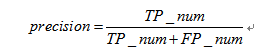
接下来我们计算准确率和召回率。准确率的计算公式是这样的:
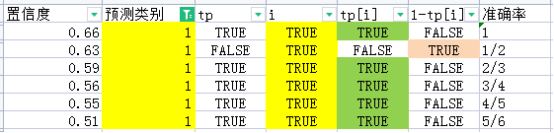
TP的数量从上面的表格可知为5,FP的数量为1,所以precision=5/(5+1)=1/6。
但是呢,这样求准曲率,是得不到AP的,因为AP是在不同置信度阈值的情况下的面积积分(稍后详细介绍面积积分)。
上面求的准确率,是以0.4位置信度阈值时求得的,但如果我卡置信度阈值为0.66(即我认为正样本不但要满足与GT的最大iou大于阈值,还要置信度大于等于0.66),那么在置信度大于等于0.66的所有预测结果中,TP的数量是1,FP的数量是0,此时precision=1/(1+0)=1;若我设定置信度阈值为0.63,那么有两个预测框符合要求,其中一个为TP,一个为FP,那么precision=1/(1+1)=1/2。
以此类推,可以求得不同置信度阈值时的准确率,结果如下:
接下来求召回率,召回率的公式是这样的:
这里FN_num表示“被错(False)当成负类的(Negative)样本”的数量,即原来是正的,却被认为是负的。
那么上面的表格里,哪些是FN呢?其实FN不在表格中,表格里只有TP和FP,而FN在GT中,GT中的边框如果被预测到了,那么就是TP,就会显示在上面的表格里,如果没有被预测到,那么就是FN。那么TP+FN的数量,其实就是验证集中GT的数量,而GT的数量,可以从验证集的标签中获得,假设它是6,那么召回率是:recall=5/6。
如果要计算AP,必须同准确率一样,要在不同置信度阈值的情况下计算一遍召回率,假设置信度阈值为0.66,那么TP的数量是1,此时recall=1/6。以此类推,可以求得不同阈值时的召回率,结果如下:
现在将准确率和召回率两列取出,并转化为小数(转小数可以方便绘图),那么有:
以召回率为横坐标,准确率为纵坐标绘制折线图:
此即为准确率和召回率的曲线图。当然,现在暂时还不能计算AP,因为recall-precision的曲线是单调递减的,而且只能为水平或竖直,不可能有斜的,所以必须对上面的图像进行调整。上面的曲线。当r=k时,的取值是r≥k时p的最大值,因此当r=0时,p=1,后面不同的r对应p也是需要重新算。调整结果如下:
r=0.17,p=1
r=0.17,p=0.83
r=0.33,p=0.83
r=0.5,p=0.83
r=0.67,p=0.83
r=0.83,p=0.83
r=0.17时之所以取两个值,是因为防止recall-precision出现斜线。按照上面的结果绘制折线图,结果如下:

加下来求曲线以下部分的面积:
1*(0.17-0)+0.83*(0.83-0.17)=0.7178
这就是c类的AP,其他类别的AP也是这么计算。
虽然类别1的AP计算完了,但是我们这里还要解读一下compute_ap函数:
在上面的表格中新增两列,分别为tpc和fpc,
tpc = (tp[i]).cumsum(),
fpc = (1 - tp[i]).cumsum(),
新增之后结果如下:
再增加两列,分别为recall_curve和precision_curve,其中:
recall_curve = tpc / (n_gt + 1e-16)
precision_curve = tpc / (tpc + fpc)
新增之后为:
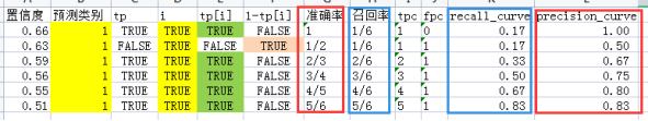
从表中可以看到,recall_curve和precision_curve分别是不同置信度阈值下的召回率和准确率。
现在我们来说一下compute_ap函数内部是如何根据recall_curve和precision_curve算出AP的。
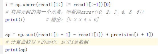
原来召回率是[0.17, 0.17, 0.33, 0.5, 0.67, 0.83],要求曲线和坐标轴围成的面积,那么必须有端点,即0和1,将这两个点补上,代码为:
r = np.concatenate(([0.0], recall, [1.0]))
补上之后recall(后面简称为r)为[0. 0.17 0.17 0.33 0.5 0.67 0.83 1. ],r多了两个端点,自然precision(后面简称为p)也要加上这两个点,代码为:
p = np.concatenate(([0.0], precision, [0.0]))
因为我们把r当成因变量,p当成因变量,所以r加两个端点很自然,一个是最小值0,另一个是最大值1,但precision两端的点就没那么简单了,这里暂时用0替代,后面还会改。
r为0时对应的p是多少呢?根据voc2010的算法(voc 2007和voc2010两个数据集诞生时,算法不一样,2010年之后,无论哪个数据集,都使用voc2010的算法了),当r=k时,的取值是r≥k时p的最大值,因此当r=0时,p=1,后面不同的r对应p也是需要重新算,最后得到的准确率数组为(在程序中是对precision进行从后往前更新,取第i和第i-1个元素中较大的值,作为第i个元素的值):
[1. 1. 0.83 0.83 0.83 0.83 0.83 0.]
在坐标系中以r为横坐标,p为纵坐标,绘制r-p折线,该折线单调递减:

计算AP的程序:
输出
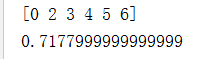
这和我们刚刚手算得到的结果基本是一致的。
(2)mAP的计算程序
在utils下面新建一个名为eva.py的文件,新建之后,目录结构如下:

们之前划分得到的验证集此时可以发挥作用了,我们的目的就是让模型在验证集上计算mAP值。
在eva.py中,先将需要的包导入进来
import tqdm
from torch.autograd import Variable
import numpy as np

from utils.datasets import ListDataset
from utils.utils import *
新建一个名为evaluate的函数,在函数中,先把模型切换到评估状态,然后再把验证集封装成数据导入器,代码如下:
def evaluate(model, path, iou_thres, conf_thres, nms_thres, img_size, batch_size):
    """

    :param model:Darknet模型对象
    :param path: 存放了验证集文件名的文件
    :param iou_thres: iou阈值,
    :param conf_thres:置信度阈值
    :param nms_thres:
    :param img_size:
    :param batch_size:
    :return:
    """
    # 把模型切换到评估模式
    model.eval()

    # Get dataloader
    dataset = ListDataset(path, img_size=img_size, augment=False, multiscale=False)
    dataloader = torch.utils.data.DataLoader(
        dataset, batch_size=batch_size, shuffle=False, num_workers=1, collate_fn=dataset.collate_fn
    )
接下来是使用模型,逐个batch进行预测,然后进行非极大值抑制:
    # Tensor = torch.cuda.FloatTensor if torch.cuda.is_available() else torch.FloatTensor
    Tensor = torch.FloatTensor      # TODO 本来应该根据model的device来选择设备,这里我们简单点

    labels = []
    sample_metrics = []  # List of tuples (TP, confs, pred)
    for batch_i, (_, imgs, targets) in enumerate(tqdm.tqdm(dataloader, desc="Detecting objects")):  # 使用tqdm打印进度条,便于观察进度
        # tqdm.tqdm(iter, desc) iter是可迭代对象,desc是描述,用于显示迭代进度

        # Extract labels
        labels += targets[:, 1].tolist()    # 抽取标签中的类别信息

        # Rescale target 转换标签值,以便后面可以和预测值进行比较
        targets[:, 2:] = xywh2xyxy(targets[:, 2:])  # boundingbox的数据原本是中心坐标和高宽,现在换成了左上角和右下角角点坐标
        targets[:, 2:] *= img_size                  # 因为boundingbox是目标值,所以将其转化为图片中的真实坐标

        imgs = Variable(imgs.type(Tensor), requires_grad=False)

        with torch.no_grad():
            outputs = model(imgs)                   # 使用模型进行预测
            outputs = non_max_suppression(outputs, conf_thres=conf_thres, nms_thres=nms_thres)  # 非极大值抑制
            # outputs是一个列表,具体看non_max_suppression方法

        # 获得当前batch中,每一张图片经过NMS之后的结果
        sample_metrics += get_batch_statistics(outputs, targets, iou_threshold=iou_thres)
上面的程序中,出现三个函数:xywh2xyxy、non_max_suppression和get_batch_statistics,在evaluate函数后面新建这三个函数。其中xywh2xyxy是目标框信息由“中心点横纵坐标和高宽”转化为“上下角点的横纵坐标”,代码如下:
def xywh2xyxy(x):
    """
    边框信息转化
    :param x: 由中心点坐标和高宽构成的边框
    :return: 由上下角点坐标构成的边框
    """
    y = x.new(x.shape)
    y[..., 0] = x[..., 0] - x[..., 2] / 2
    y[..., 1] = x[..., 1] - x[..., 3] / 2
    y[..., 2] = x[..., 0] + x[..., 2] / 2
    y[..., 3] = x[..., 1] + x[..., 3] / 2
    return y
接下来是非极大值抑制,这个函数的设计思路比较复杂,首先将置信度大于阈值的“目标”筛选出来,然后对“目标”的维度进行整理,即将类别概率值转化为最大值及其类别编号,然后把相同类别中,与置信度最大的预测框的iou大于阈值的预测框筛选出来,这些即为要抑制的预测框,这个听起来有点拗口,具体看下面的程序会很清晰。值得注意的是,被抑制的预测框并非毫无用处,最后保留的预测框也不是置信度最大的那个,而是所有大于iou阈值的预测框经过置信度加权得到的,详见下面的代码:
def non_max_suppression(prediction, conf_thres=0.5, nms_thres=0.4):
    """
    Removes detections with lower object confidence score than 'conf_thres' and performs
    Non-Maximum Suppression to further filter detections.
    Returns detections with shape:
        (x1, y1, x2, y2, object_conf, class_score, class_pred)
    :param prediction: 维度为(batch_size, number_pred, 85),number_pred是三个检测头的数量之和
    :param conf_thres: 置信度阈值
    :param nms_thres: 非极大值抑制时的iou阈值
    :return: 输出一个列表,列表中的元素,要么为None,要么是维度为(num_obj, 7)的张量
    """

    # From (center x, center y, width, height) to (x1, y1, x2, y2)
    prediction[..., :4] = xywh2xyxy(prediction[..., :4])        # 将预测得到的boundingbox标签转化为两个个角点的坐标
    output = [None for _ in range(len(prediction))]             # 先获得由若干None构成的列表
    for image_i, image_pred in enumerate(prediction):
        # Filter out confidence scores below threshold
        image_pred = image_pred[image_pred[:, 4] >= conf_thres]     # 先筛选置信度大于阈值的预测框
        # If none are remaining => process next image
        if not image_pred.size(0):         # 如果当前图片中,所有目标的置信度都小于阈值,那么就进行下一轮循环
            continue
        # Object confidence times class confidence
        score = image_pred[:, 4] * image_pred[:, 5:].max(1)[0]
        # image_pred[:, 4]是置信度,image_pred[:, 5:].max(1)[0]是概率最大的类别索引

        # Sort by it
        image_pred = image_pred[(-score).argsort()]
        # argsort()是将(-score)中的元素从小到大排序,返回排序后索引
        # 将(-score)中的元素从小到大排序,实际上是对score从大到小排序
        # 将排序后的索引放入image_pred中作为索引,实际上是对本张图片中预测出来的目标进行排序

        class_confs, class_preds = image_pred[:, 5:].max(1, keepdim=True)   #
        detections = torch.cat((image_pred[:, :5], class_confs.float(), class_preds.float()), 1)
        # 经过上条命令之后,detections的维度为(number_pred, 7),
        # 前4列是边框的左上角点和右下角点的坐标,第5列是目标的置信度,第6列是类别置信度的最大值,
        # 第7列是类别置信度最大值所对应的类别

        # Perform non-maximum suppression
        keep_boxes = []     # 用来存储符合要求的目标框

        while detections.size(0):   # 如果detections中还有目标
            large_overlap = bbox_iou(detections[0, :4].unsqueeze(0), detections[:, :4]) > nms_thres
            # bbox_iou(detections[0, :4].unsqueeze(0), detections[:, :4])返回值的维度为(num_objects, )
            # bbox_iou的返回值与非极大值抑制的阈值相比较,获得布尔索引
            # 即剩下的边框中,只有detection[0]的iou大于nms_thres的,才抑制,即认为这些边框与detection[0]检测的是同一个目标

            label_match = detections[0, -1] == detections[:, -1]
            # 布尔索引,获得所有与detection[0]相同类别的对象的索引

            # Indices of boxes with lower confidence scores, large IOUs and matching labels
            invalid = large_overlap & label_match   # &是位运算符,两个布尔索引进行位运算
            # 上面位运算得到的索引,是所有应该被抑制的边框的索引,即无效索引
            # 所谓无效索引,即和最大置信度边框有相同类别,而且有比较高的交并比的边框的索引
            # 这里是筛选出无效边框,只有被筛选出来的边框才需要被抑制

            weights = detections[invalid, 4:5]      # 根据无效索引,获得被抑制边框的置信度

            # 加权获得最后的边框坐标
            detections[0, :4] = (weights * detections[invalid, :4]).sum(0) / weights.sum()
            # 上面的命令是将当前边框,和被抑制的边框,进行加权,类似于好几个边框都检测到了同一张人脸,
            # 将这几个边框的左上角点横坐标x进行加权(按照置信度加权),获得最后边框的x
            # 对左上角点的纵坐标y,以及右下角点的横纵坐标也进行加权处理

            keep_boxes += [detections[0]]       # 将有效边框加入到 keep_boxes 中
            detections = detections[~invalid]   # 去掉无效边框,更新detections

        if keep_boxes:  # 如果keep_boxes不是空列表
            output[image_i] = torch.stack(keep_boxes)   # 将目标堆叠,然后加入到列表
            # 假设NMS之后,第i张图中有num_obj个目标,那么torch.stack(keep_boxes)的结果是就是一个(num_obj, 7)的张量,没有图片索引

        # 如果keep_boxes为空列表,那么output[image_i]则未被赋值,保留原来的值(原来的为None)

    return output
现在我们来说一下get_batch_statistics,这个函数起的名字不太恰当,因为他的意义仅仅是解码,在前面介绍mAP的原理中,相当于求下面图中的数据:

具体代码如下:
def get_batch_statistics(outputs, targets, iou_threshold):
    """
    outputs是模型的预测结果,但预测的边框未必都合格,必须从中筛选出合格的边框,所谓合格,
    就是预测框和真实框的iou大于阈值,这里仅仅考虑iou,不考虑预测类别是否相同
    :param outputs:一个列表,列表中第i个元素,要么是维度为(num_obj, 7)的张量(第i张图片的预测结果),
                    要么是None(即模型认为该张图片中没有目标)
    :param targets:一个张量,这个张量的首列是图片在batch中的索引,第2列是类别标签,
                后面4列分别是box的上下角点横纵坐标
    :param iou_threshold:预测的边框与GT的阈值,经过NMS之后,留下的边框必须与GT的iou超过这个阈值才能参与评价
    :return:[A, B, C,……],  A、B、C都是列表,他们分别代表包含了合格预测框的图片
            列表A由三个元素组成,即[true_positives, pred_scores, pred_labels],列表B,C也是如此
            true_positives 一维张量,代表当前图片的所有预测边框中,合格边框的布尔索引
            pred_scores 一维张量,代表当前图片的所有预测边框的置信度,
            pred_labels 一维张量,代表当前图片的所有预测边框的类别标签
    """
    """ Compute true positives, predicted scores and predicted labels per sample """
    batch_metrics = []
    for sample_i in range(len(outputs)):
        # sample_i是图片索引

        if outputs[sample_i] is None:
            continue

        output = outputs[sample_i]      # 获取第i张图片的预测结果
        pred_boxes = output[:, :4]      # 从输出中获得预测框的上下角点的坐标
        pred_scores = output[:, 4]      # 获得置信度
        pred_labels = output[:, -1]     # 获得类别索引

        true_positives = np.zeros(pred_boxes.shape[0])  # TP,即真实正样本,详情要看后面的循环
        # pred_boxes.shape[0]是第i张图片中的目标数量

        annotations = targets[targets[:, 0] == sample_i][:, 1:]
        # 从目标张量中获得第i张图片的标签
        # 从之所以从1开始,是因为0是图片索引,这里是遍历图片,所以不需要图片索引

        target_labels = annotations[:, 0] if len(annotations) else []
        # 获取目标的类别索引,若图片中无目标则返回空列表
        # targets和output的排列方式不一样,targets中第一列是图片索引,第二列是类别索引

        if len(annotations):
            detected_boxes = []                 # 用来存储预测合格的边框的索引,
            # 所谓预测合格,是指与GT的iou大于阈值
            target_boxes = annotations[:, 1:]   # 从标签中获得边框的信息

            for pred_i, (pred_box, pred_label) in enumerate(zip(pred_boxes, pred_labels)):
                # zip(pred_boxes, pred_labels)是每次分别从pred_boxes和pred_labels中抽取一个元素组成元组

                # If all targets are found break
                if len(detected_boxes) == len(annotations):
                    # 当条件成立时,说明标签中的目标边框已经被匹配完,可以跳出循环了
                    # 另外一种结束循环的方法是zip(pred_boxes, pred_labels)被遍历完
                    break

                # Ignore if label is not one of the target labels
                if pred_label not in target_labels:
                    # 说明类别预测错误
                    continue

                iou, box_index = bbox_iou(pred_box.unsqueeze(0), target_boxes).max(0)
                # pred_box.unsqueeze(0)之后,pred_box的维度为(1, 4),
                # target_boxes的维度为 (num_obj, 4)
                # bbox_iou(pred_box.unsqueeze(0), target_boxes)的返回值是pred_box与当前图片中所有GT的iou
                # 选择最大的iou及其在targets中的索引

                if iou >= iou_threshold and box_index not in detected_boxes:
                    # 如果最大的iou大于阈值,且这个边框对应的GT索引不在detected_boxes中,
                    # 那么就将这个边框对应的GT索引加入到detected_boxes中,并在TP中将对应的位置标1

                    detected_boxes += [box_index]
                    true_positives[pred_i] = 1

        # 经过上面的循环后true_positives的元素个数,表示的是模型预测有多少个目标,
        # 这些预测的目标如果合格(与targets的最大iou大于阈值),就在对应位置标1,否则保留原来的值(即为0)
        # true_positives可以作为pred_scores和pred_labels的布尔索引

        # 将当前图片的true_positives,pred_scores, pred_labels加入到batch_metrics中
        batch_metrics.append([true_positives, pred_scores, pred_labels])

    return batch_metrics
让我们回到evaluate函数中,把get_batch_statistics的结果进行级联,然后计算mAP,程序如下:
    # Concatenate sample statistics
    L = [np.concatenate(x, 0) for x in list(zip(*sample_metrics))]  # x每次获得的都是一个元组,
    # sample_metrics是一个大列表,其中每个元素都是一个小列表
    # 每次获得的x都是从小列表中抽取一个元素(该元素是张量),构成的一个元组
    # x是元组里面套了若干个张量(有多少个batch,就有多少个张量)
    # np.concatenate是将这几个张量进行级联,相当于原来目标是分散在各个batch中,现在组合在在一起
    # 最后的结果是L里面套了三个numpy数组,分别是true_positives,pred_scores和pred_labels
    # 这三个数组都是代表了整个验证集,而非仅仅单个batch

    print(len(L))
    true_positives, pred_scores, pred_labels = L[0], L[1], L[2]

    # true_positives, pred_scores, pred_labels都是numpy数组
    # 这里求统计指标时,就不再是一个batch一个batch地求了,而是在整个验证集上求
    precision, recall, AP, f1, ap_class = ap_per_class(true_positives, pred_scores, pred_labels, labels)

    return precision, recall, AP, f1, ap_class
这里调用了ap_per_class的函数,这是计算每个类别的AP值的函数,需要在后面新增。这部分程序的理解,要和前面介绍“mAP的计算原理”的部分结合起来,才比较容易弄懂,特别是使用recall_curve和precision_curve计算AP(这里还另外调用了compute_ap函数,后面会介绍)。代码如下:
def ap_per_class(tp, conf, pred_cls, target_cls):
    """ Compute the average precision, given the recall and precision curves.
    Source: https://github.com/rafaelpadilla/Object-Detection-Mricset.
    # Arguments
        tp:    一维数组
        conf:  一维数组
        pred_cls: 一维数组
        target_cls: 一维数组
    # Returns
        The average precision as computed in py-faster-rcnn.
    """

    # Sort by objectness
    i = np.argsort(-conf)   # 将conf从大到小排序,返回排序后的索引
    tp, conf, pred_cls = tp[i], conf[i], pred_cls[i]    # 将tp, conf, pred_cls从大到小排序

    # Find unique classes
    unique_classes = np.unique(target_cls)     # 将当前batch中所有GT的类别信息进行去重

    # Create Precision-Recall curve and compute AP for each class
    ap, p, r = [], [], []
    for c in tqdm.tqdm(unique_classes, desc="Computing AP"): # 这个循环是计算每个类别的AP值
        i = pred_cls == c               # 返回布尔值,即是否为当前类别
        n_gt = (target_cls == c).sum()  # Number of ground truth objects
        n_p = i.sum()                   # Number of predicted objects

        if n_p == 0 and n_gt == 0:
            # 如果当前类别的GT和预测框的数量同时为0,
            # 这种情况基本不可能发生,因为c的来源就是GT,至少GT不可能等于0
            continue
        elif n_p == 0 or n_gt == 0:     #
            ap.append(0)
            r.append(0)
            p.append(0)
        else:
            # Accumulate FPs and TPs
            fpc = (1 - tp[i]).cumsum()
            # tp本来就是合格边框的布尔索引,经过i又一轮筛选后,就成为了当前类别的合格边框的布尔索引
            # (1 - tp[i]).cumsum() 先进行广播,再计算轴向元素累加和

            tpc = (tp[i]).cumsum()          # 将当前类别的布尔索引进行累加 结果可能是0,1,1,4

            # Recall
            recall_curve = tpc / (n_gt + 1e-16)     # 召回率曲线计算
            r.append(recall_curve[-1])              # recall_curve[-1]是不设置信度阈值时的召回率

            # Precision
            precision_curve = tpc / (tpc + fpc)     # 准确率曲线计算
            p.append(precision_curve[-1])           # precision_curve[-1]是不设置信度阈值时的准确率

            # AP from recall-precision curve
            ap.append(compute_ap(recall_curve, precision_curve))

    # Compute F1 score (harmonic mean of precision and recall)
    p, r, ap = np.array(p), np.array(r), np.array(ap)       # 将准确率、召回率、AP做成numpy数组
    f1 = 2 * p * r / (p + r + 1e-16)                        # 求F1分数

    # 返回统计指标
    # 这里之所以要把unique_classes一起返回,因为p[i], r[i], ap[i]等统计指标,
    # 是和unique_classes[i]表示的类别对应的
    return p, r, ap, f1, unique_classes.astype("int32")
这里出现compute_ap函数,在ap_per_class后面加上,这段代码的理解,同样需要结合“mAP的计算原理”代码如下:
def compute_ap(recall, precision):
    """ Compute the average precision, given the recall and precision curves.
    Code originally from https://github.com/rbgirshick/py-faster-rcnn.

    # Arguments
        recall:    The recall curve (list).
        precision: The precision curve (list).
    # Returns
        The average precision as computed in py-faster-rcnn.
    """
    # correct AP calculation
    # first append sentinel values at the end
    mrec = np.concatenate(([0.0], recall, [1.0]))
    mpre = np.concatenate(([0.0], precision, [0.0]))

    # compute the precision envelope
    for i in range(mpre.size - 1, 0, -1):
        mpre[i - 1] = np.maximum(mpre[i - 1], mpre[i])

    # to calculate area under PR curve, look for points
    # where X axis (recall) changes value
    i = np.where(mrec[1:] != mrec[:-1])[0]
    # np.where(condition)表示找到符合条件的索引

    # and sum (\Delta recall) * prec
    ap = np.sum((mrec[i + 1] - mrec[i]) * mpre[i + 1])
    return ap
(3)在训练中添加模型的评价
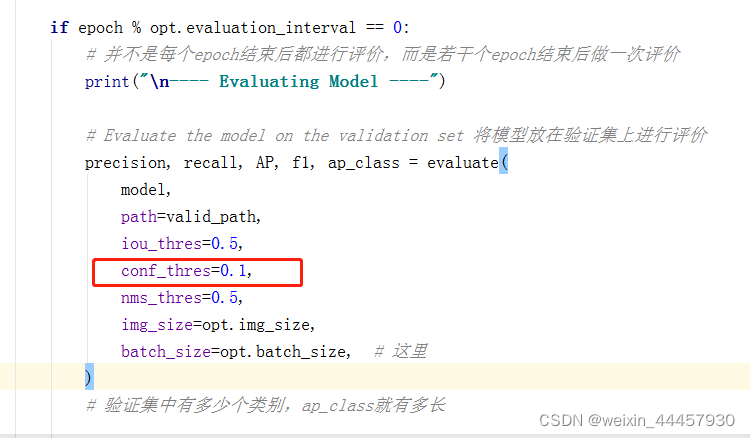
让我们回到train.py中,我们每训练若干epoch,就对模型进行一次评价,代码如下:
        if epoch % opt.evaluation_interval == 0:
            # 并不是每个epoch结束后都进行评价,而是若干个epoch结束后做一次评价
            print("\n---- Evaluating Model ----")

            # Evaluate the model on the validation set 将模型放在验证集上进行评价
            precision, recall, AP, f1, ap_class = evaluate(
                model,
                path=valid_path,
                iou_thres=0.5,
                conf_thres=0.5,
                nms_thres=0.5,
                img_size=opt.img_size,
                batch_size=opt.batch_size,  # 这里
            )
            # 验证集中有多少个类别,ap_class就有多长

            # 将各个类别的评价指标的平均值写入log,
            # 注意,这里是整个验证集上的平均值,而不是单个batch上的平均值
            evaluation_metrics = [
                ("val_precision", precision.mean()),
                ("val_recall", recall.mean()),
                ("val_mAP", AP.mean()),
                ("val_f1", f1.mean()),
            ]
            logger.list_of_scalars_summary(evaluation_metrics, epoch)

            # Print class APs and mAP
            ap_table = [["Index", "Class name", "AP"]]
            for i, c in enumerate(ap_class):
                ap_table += [[c, class_names[c], "%.5f" % AP[i]]]
            print(AsciiTable(ap_table).table)
            print(f"---- mAP {AP.mean()}")
于此同时,我们还要看一下是否达到了模型的保存点(因为同样是每隔若干个epoch保存一次模型),如果到了保存点,那么就保存。我们这里为了方便演示,我们就训练一个epoch就退出循环。
        if epoch % opt.checkpoint_interval == 0:
            # 保存模型
            torch.save(model.state_dict(), f"checkpoints/yolov3_ckpt_%d.pth" % epoch)

        # 我们这里也是仅仅进行一个epoch进行演示
        break
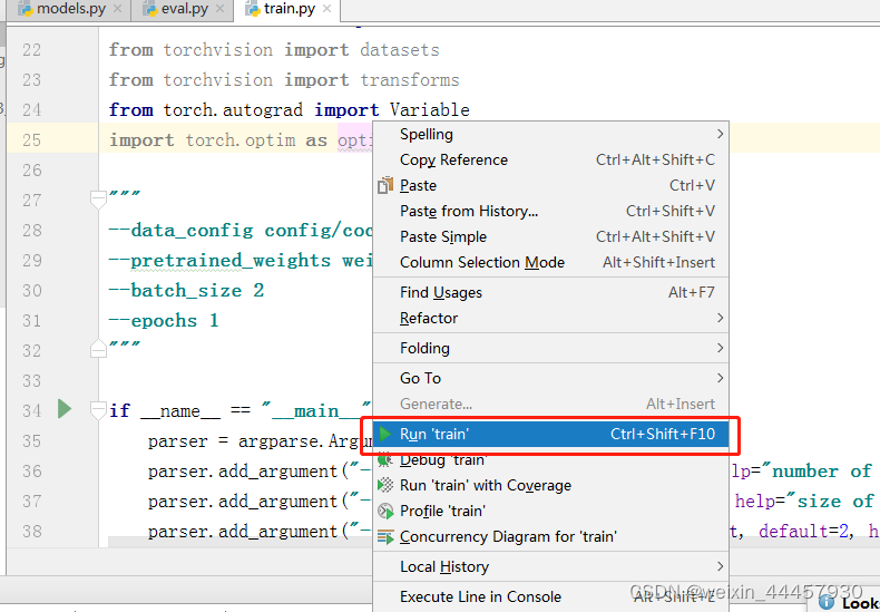
最后运行train.py,相对应的命令行参数为:
--data_config config/coco.data
--pretrained_weights weights/darknet53.conv.74
--batch_size 2
--epochs 1
在pycharm中,可以用如下方式添加命令行参数:Run->Edit Configurations

在弹出的对话框中点击python

在右边的script path中添加脚本路径

将参数复制到 Parameters中:

名字和项目也要改

现在可以按照普通的Python程序运行了
上面的程序很可能报下面的错误:

报这种错误有两种情况,一种情况是图片中压根就不存在目标,另一种情况是训练不够充分(因为只有128张图片,同时只有一个epoch),模型不够成熟,导致未能从图片中检测出目标。而当一个batch中一个目标都没有检出时,就会报这种错误。本篇博客是第二种情况,即存在目标但没能检测出来,由于我们在评估模型时,指定了shuffle=False,这样就和本篇博客中的情况一样了。我们可以把评估参数中的置信度阈值改小,比如改成0.1,使更多的目标能够得到保留:
OK,此时就可以得到正常输出了:
---- Evaluating Model ----
Detecting objects:   0%|          | 0/5 [00:00<?, ?it/s]2021-12-13 10:43:48.310192: W tensorflow/stream_executor/platform/default/dso_loader.cc:55] Could not load dynamic library 'cudart64_101.dll'; dlerror: cudart64_101.dll not found
2021-12-13 10:43:48.310192: I tensorflow/stream_executor/cuda/cudart_stub.cc:29] Ignore above cudart dlerror if you do not have a GPU set up on your machine.
Detecting objects: 100%|██████████| 5/5 [00:25<00:00,  5.09s/it]
3
Computing AP: 100%|██████████| 20/20 [00:00<00:00, 9999.53it/s]
+-------+--------------+---------+
| Index | Class name   | AP      |
+-------+--------------+---------+
| 0     | person       | 0.00000 |
| 1     | bicycle      | 0.00000 |
| 2     | car          | 0.00000 |
| 4     | aeroplane    | 0.00000 |
| 5     | bus          | 0.00000 |
| 7     | truck        | 0.00000 |
| 11    | stop sign    | 0.00000 |
| 16    | dog          | 0.00000 |
| 22    | zebra        | 0.00000 |
| 25    | umbrella     | 0.00000 |
| 26    | handbag      | 0.00000 |
| 27    | tie          | 0.00000 |
| 36    | skateboard   | 0.00000 |
| 41    | cup          | 0.00000 |
| 42    | fork         | 0.00000 |
| 53    | pizza        | 0.00000 |
| 56    | chair        | 0.00000 |
| 60    | diningtable  | 0.00000 |
| 72    | refrigerator | 0.00000 |
| 74    | clock        | 0.00000 |
+-------+--------------+---------+
---- mAP 0.0
当然,虽然有输出,但mAP还是0,估计是和


 4022
4022


 被折叠的 条评论
为什么被折叠?
被折叠的 条评论
为什么被折叠?
 到【灌水乐园】发言


