透射投影矩阵的线性与非线性估计，Levenberg Marquardt 算法应用（非线性估计），附代码／数据

背景知识简介

在计算机视觉中，有一块领域叫做相机标定，这篇博客主要描述的是相机标定中，通过对应的3d点坐标（世界坐标系，World Frame）和2d点坐标（图像坐标系，Image Frame）透射投影。

什么是透射投影

我们需要把3d点$(x_W,y_W,z_W,1)$的坐标从世界坐标系（World Frame）转化到图像坐标系（Image Frame）$(x_I,y_I,w_I)$。这里使用的都是齐次坐标（Homogeneous Coordinates），主要的目的就是可以把旋转和位移放到同一个矩阵中，想要进一步了解的同学可以自行百度。
$$\left[\begin{array}{c}{x}_I\\ y_I\\ w_I\end{array}\right]=\left[\begin{array}{ccc}{R}^{3\times 3}& |& t^{3\times 1}\end{array}\right]\left[\begin{array}{c}{x}_w\\ y_w\\ z_w\\ 1\end{array}\right]=P\left[\begin{array}{c}{x}_w\\ y_w\\ z_w\\ 1\end{array}\right]$$
这里的$P^{3\times 4}$就是我们需要的透射投影矩阵（Projection Matrix）。其中$R^{3\times 3}$是一个旋转矩阵，我们可以理解为它表示了一个3d点绕着x,y,z轴分别旋转了$\alpha ,\theta ,\gamma$度，所以虽然它包含了9个元素（$3\times 3=9$），但是它只有3个自由度（3 DoFs，Degree of Freedom）。然后$t$可以视为一个位移，它包含3个元素且自由度为3（3 DoFs）。所以整个透射投影矩阵（Projection Matrix）$P$虽然包含12（$3\times 4=12$）个未知元素，但是它的的自由度为6，也就是说，最少我们需要6组对应的3d点和2d点才能对它进行估计（可以简单理解为至少需要6个方程才能解6个未知数）。

p.s. 这里我们不进一步讨论矫正矩阵(Calibration Matrix)、正准矩阵（Canonical Matrix）等概念。

线性估计（Direct Linear Transformation (DLT) Algorithm）

理论推导分析

我们现在有的数据集为n组对应点， { ( x i , X i )  for  i = 0 , 1 , 2 , . . . , n } \{(x_i,X_i) \text{ for } i = 0,1,2, ... ,n \} {(xi​,Xi​) for i=0,1,2,...,n} 其中 $x=(x_I/w_I,y_I/w_I,1)$ $X=(x_W,y_W,z_W,1)$
$$x=PX$$
很容易，我们会联想到使用线性代数的知识$x\times x=x\times (PX)=0$（这里的乘号代表叉乘）。但是这并不是实际过程中工程师将会用的方法，具体为什么我不太记得了，希望知道的朋友可以在博客下面回复补充。现实中，工程师将使用如下等式
$$[x{]}^{\perp }x=[x{]}^{\perp }PX=\left[\begin{array}{c}{l}_1^T\\ l_2^T\end{array}\right]PX=0$$
$[x{]}^{\perp }$ 代表了相交与于$x$点两条直线$l_1^{3\times 1}$和$l_2^{3\times 1}$ (使用了引理：若$x$为直线$l$上一点，那么$x^{T}l=l^{T}x=0$)

下面我们会进行一系列推到，将$[x{]}^{\perp }PX=0$转化为一个更加方便计算估计$P$的表达式。

假设
$$P=\left[\begin{array}{cccc}{p}_{11}& p_{12}& p_{13}& p_{14}\\ p_{21}& p_{22}& p_{23}& p_{24}\\ p_{31}& p_{32}& p_{33}& p_{34}\end{array}\right]=\left[\begin{array}{c}{p}^{1T}\\ p^{2T}\\ p^{3T}\end{array}\right]$$
$$p=\text{vec}(P^T)=\left[\begin{array}{c}{p}_{11}\\ p_{12}\\ p_{13}\\ ⋮\\ p_{34}\end{array}\right]$$
$$l=\left[\begin{array}{c}a\\ b\\ c\end{array}\right]$$
那么
$$[x{]}^{\perp }PX=\left[\begin{array}{c}{l}_1^T\\ l_2^T\end{array}\right]PX=\left[\begin{array}{ccc}{a}_1& b_1& c_1\\ a_2& b_2& c_2\end{array}\right]\left[\begin{array}{c}{p}^{1T}X\\ p^{2T}X\\ p^{3T}X\end{array}\right]=\left[\begin{array}{ccc}{a}_1{X}^T& b_1{X}^T& c_1{X}^T\\ a_2{X}^T& b_2{X}^T& c_2{X}^T\end{array}\right]\left[\begin{array}{c}{p}_{11}\\ p_{12}\\ p_{13}\\ ⋮\\ p_{34}\end{array}\right]$$
因此
$$[x{]}^{\perp }PX=\left[\begin{array}{c}{l}_1^T\otimes X^T\\ l_2^T\otimes X^T\end{array}\right]p=([x{]}^{\perp }\otimes X^T)p=0$$
我们可以把n组数据写成一个大型的矩阵方程
$$\left[\begin{array}{c}[x_1{]}^{\perp }\otimes X_1^T\\ [x_2{]}^{\perp }\otimes X_2^T\\ ⋮\\ [x_n{]}^{\perp }\otimes X_n^T\end{array}\right]p=Ap=0\text{ where n≥6 }$$
至于解这个$Ap=0$的方程，最直接、有效的方法就是对矩阵$A$使用非满秩（当$n>6$）的SVD分解
$$A=U\Sigma V^T=U^{2n\times 2n}{\Sigma }^{2n\times 12}\left[\begin{array}{c}{v}^{1T}\\ v^{2T}\\ ⋮\\ v^{nT}\end{array}\right]$$
$$p^{12\times 1}=v^n$$
$p$的线性估计结果为矩阵$V$的最后一列或$V^T$的最后一行（不同的python扩展包中SVD分解的结果中可能是$V$也可能是$V^T$，请仔细看函数介绍）。

python代码实现

数据可以点击这里下载

import numpy as np
import time

def Homogenize(x):
    # converts points from inhomogeneous to homogeneous coordinates
    return np.vstack((x,np.ones((1,x.shape[1]))))


def Dehomogenize(x):
    # converts points from homogeneous to inhomogeneous coordinates
    return x[:-1]/x[-1]


def Normalize(pts):
    # data normalization of n dimensional pts
    #
    # Input:
    #    pts - is in inhomogeneous coordinates
    # Outputs:
    #    pts - data normalized points
    #    T - corresponding transformation matrix
    """your code here"""
    pts_mean = pts.sum(1)/pts.shape[1]  ## mean of pts
    pts_var = np.var(pts, axis=1).sum() ## var = x_var + y_var (+ z_var)
    s = (pts.shape[0]/pts_var)**0.5
    T = np.eye(pts.shape[0]+1)
    for i in range(pts.shape[0]):
        T[i,i] = s
    T[:,-1] = Homogenize((-pts_mean * s).reshape(-1,1)).flatten()
    pts = np.dot(T,Homogenize(pts))
    return pts, T

def ComputeCost(P, x, X):
    # Inputs:
    #    x - 2D inhomogeneous image points
    #    X - 3D inhomogeneous scene points
    #
    # Output:
    #    cost - Total reprojection error
    n = x.shape[1]
    covarx = np.eye(2*n)
    
    """your code here"""
    X = Homogenize(X)
    x_project = np.dot(P,X)
    x_proj = Dehomogenize(x_project)
    cost = ((x-x_proj)**2).sum()
    
    return cost

def GetPeprp(x):
    # Inputs:
    #    x - 2D homogeneous image points, 3*n
    # Output:
    #    x_perp - perpendicular complement of x, 2n*3
    
    n = x.shape[1]
    x_perp = np.zeros((2*n,3))
    for i in range(2*n):
        if i%2 == 0:
            x_perp[i,0] = 1
        else:
            x_perp[i,1] = 1
    x_inhomo = Dehomogenize(x)
    x_perp[:,-1] = -x_inhomo.T.flatten()
    
    return x_perp

def DLT(x, X, normalize=True):
    # Inputs:
    #    x - 2D inhomogeneous image points
    #    X - 3D inhomogeneous scene points
    #    normalize - if True, apply data normalization to x and X
    #
    # Output:
    #    P - the (3x4) DLT estimate of the camera projection matrix
    P = np.eye(3,4)+np.random.randn(3,4)/10
        
    # data normalization
    if normalize:
        x, T = Normalize(x)
        X, U = Normalize(X)
    else:
        x = Homogenize(x)
        X = Homogenize(X)
    
    """your code here"""
    x_perp = GetPeprp(x)
    n = x.shape[1]
    A = np.zeros((2*n, 12))  ## (2n,12)
    for i in range(n):
        for j in range(3):
            A[2*i,4*j:4*j+4] = x_perp[2*i,j]*X[:,i]
            A[2*i+1,4*j:4*j+4] = x_perp[2*i+1,j]*X[:,i]
    
    _, _ , Vh = np.linalg.svd(A)
    P = Vh[-1].reshape(3,4)
    
    # data denormalize
    if normalize:
        P = np.linalg.inv(T) @ P @ U
        
    P = P/np.linalg.norm(P)
    return P
    
# load the data
x=np.loadtxt('points2D.txt').T
X=np.loadtxt('points3D.txt').T


# compute the linear estimate without data normalization
print ('Running DLT without data normalization')
time_start=time.time()
P_DLT = DLT(x, X, normalize=False)
cost = ComputeCost(P_DLT, x, X)
time_total=time.time()-time_start
# display the results
print('took %f secs'%time_total)
print('Cost=%.9f'%cost)


# compute the linear estimate with data normalization
print ('Running DLT with data normalization')
time_start=time.time()
P_DLT = DLT(x, X, normalize=True)
cost = ComputeCost(P_DLT, x, X)
time_total=time.time()-time_start
# display the results
print('took %f secs'%time_total)
print('Cost=%.9f'%cost)

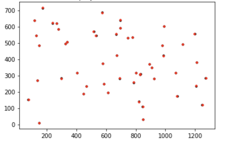
大家可以自行写一下plot结果的部分，差不多会是这样，黑色的是真实2d点，红色的是根据线性估计计算出的$P$计算出的投影点。

代码中引入了归一化（Normalization）的概念，可以有效地降低参数估计中的误差。具体的公式可以从代码中推出，这里就不一一展开了。

非线性估计

Levenberg Marquardt 算法介绍

给定条件：

1. 度量矢量 (Measurement Vector) $x$和它的协方差${\Sigma }_x$
2. 参数矢量 (Parameter Vector) $\hat{P}$（始化估计）

目标：

1. 寻找到 $\hat{P}$最小化${ϵ}^T{\Sigma }_x^{-1}ϵ$，其中$ϵ=x-\hat{x}$，$\hat{x}$为使用估计的参数获得的度量。

具体算法：

1. $\lambda =0.001,ϵ=x-\hat{x}$
2. 计算Jacobian矩阵$J=\frac{\partial \hat{x}}{\partial P}$
3. 加权最小二乘法方程： $(J^T{\Sigma }_x^{-1}J)\delta =J^T{\Sigma }_x^{-1}ϵ$，这条方程从$J\delta =ϵ$中获得。
4. 增广方程：$(J^T{\Sigma }_x^{-1}J+\lambda I)\delta =J^T{\Sigma }_x^{-1}ϵ$，求解$\delta$。值得注意的是，这里的$(J^T{\Sigma }_x^{-1}J+\lambda I)$是一个对称矩阵。
5. 获得候选参数矢量：${\hat{P}}_0=\hat{P}+\delta$
6. ${\hat{P}}_0\to {\hat{x}}_0,{ϵ}_0=x-{\hat{x}}_0$
7. 判定：如果${ϵ}_0{\Sigma }_x^{-1}{ϵ}_0$小于$ϵ{\Sigma }_x^{-1}ϵ$，则$\hat{P}={\hat{P}}_0,ϵ={ϵ}_0,\lambda =0.1\lambda$，回到步骤2，并记一次迭代；反之，$\lambda =10\lambda$，回到步骤4，不计入迭代次数。

（未完待续…）