


 本文介绍了如何使用R语言中的三种方法处理数据集中的缺失值,包括内置函数的简单插补、MICE包和missForest插补。通过实例分析了在Titanic数据集中应用这些方法的效果,展示了它们对数据分布的影响。
Nhanes美国营养调查数据库的培训课程来了!
现实生活中我们遇到的数据通常是杂乱无章并且有很多缺失值的,这样就使得我们要花费很多的时间和精力在数据清洗和数据准备上。因此,今天我们一起学习使用R进行数据插补的3种方法,希望可以为你以后的数据清洗节省时间。
今天介绍三种R常用的数据插补方法:1. R内置函数的简单值插补;2.MICE包插补缺失值;3.使用 missForest 包进行插补。使用到的数据集是Titanic。
1library(ggplot2)
2library(dplyr)
3library(titanic)
4library(cowplot)
5library(titanic)
首先查看一下数据集:
本篇推文以titanic_train数据集的Age变量为例进行填补,查看Age变量:
1titanic_train$Age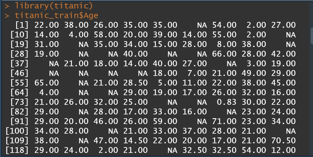
可看到有较多的缺失。在进行数据插补之前,我们先看一下要填补数据的分布:
1library(ggplot2)
2ggplot(titanic_train, aes(Age)) +
3  geom_histogram(color = "#000000", fill = "#0099F8") +
4  ggtitle("Variable distribution") +
5  theme_classic() +
6  theme(plot.title = element_text(size = 18))
注意,这里查看数据分布的目的是为了对比数据插补前后的分布是否一致。接下来我们开始插补。
1. R内置函数的简单值插补
简单插补可以用(1)任意常数插补:用0或其他数据插补;(2)均数插补;(3)中位数插补,代码如下:
1value_imputed <- data.frame(
2  original = titanic_train$Age,
3  imputed_zero = replace(titanic_train$Age, is.na(titanic_train$Age), 0),
4  imputed_mean = replace(titanic_train$Age, is.na(titanic_train$Age), mean(titanic_train$Age, na.rm = TRUE)),
5  imputed_median = replace(titanic_train$Age, is.na(titanic_train$Age), median(titanic_train$Age, na.rm = TRUE))
6)
7value_imputed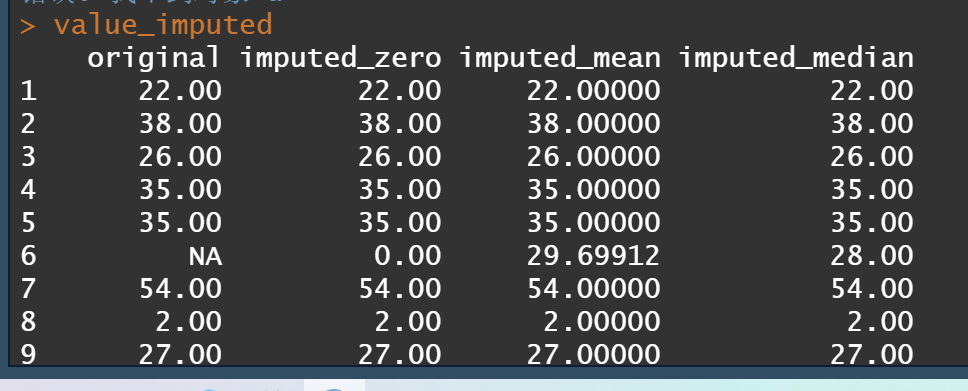
接着我们看一下插补之后数据分布是否有变化,代码如下:
1h1 <- ggplot(value_imputed, aes(x = original)) +
 2  geom_histogram(fill = "#ad1538", color = "#000000", position = "identity") +
 3  ggtitle("Original distribution") +
 4  theme_classic()
 5h2 <- ggplot(value_imputed, aes(x = imputed_zero)) +
 6  geom_histogram(fill = "#15ad4f", color = "#000000", position = "identity") +
 7  ggtitle("Zero-imputed distribution") +
 8  theme_classic()
 9h3 <- ggplot(value_imputed, aes(x = imputed_mean)) +
10  geom_histogram(fill = "#1543ad", color = "#000000", position = "identity") +
11  ggtitle("Mean-imputed distribution") +
12  theme_classic()
13h4 <- ggplot(value_imputed, aes(x = imputed_median)) +
14  geom_histogram(fill = "#ad8415", color = "#000000", position = "identity") +
15  ggtitle("Median-imputed distribution") +
16  theme_classic()
17
18plot_grid(h1, h2, h3, h4, nrow = 2, ncol = 2)
19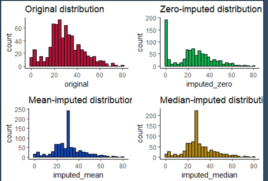
可以看到以上三种填补均对数据分布产生严重的影响。因此这种方法不是很好。
2.使用 MICE 包插补缺失值
MICE 包填补假定缺失值是随机缺失的 (MAR),该算法背后的基本思想是将每个具有缺失值的变量视为回归中的因变量,将其并他变量视为独立变量(预测变量)。
MICE包提供了许多单变量插补方法,但我们只使用少数几种。首先将所需要的变量从titanic_train数据集挑选出来:
1library(mice)
2titanic_numeric <- titanic_train %>%
3  select(Survived, Pclass, SibSp, Parch, Age)
4md.pattern(titanic_numeric)#数据缺失可视化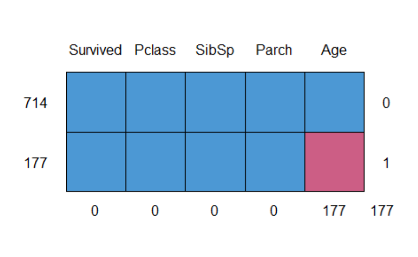
现在进行插补,我们将使用以下 MICE 插补方法:
(1)pmm:预测均值匹配;(2)cart:分类和回归树;(3)laso.norm:Lasso线性回归。
1mice_imputed <- data.frame(
2  original = titanic_train$Age,
3  imputed_pmm = complete(mice(titanic_numeric, method = "pmm"))$Age,
4  imputed_cart = complete(mice(titanic_numeric, method = "cart"))$Age,
5  imputed_lasso = complete(mice(titanic_numeric, method = "lasso.norm"))$Age
6)
7mice_imputed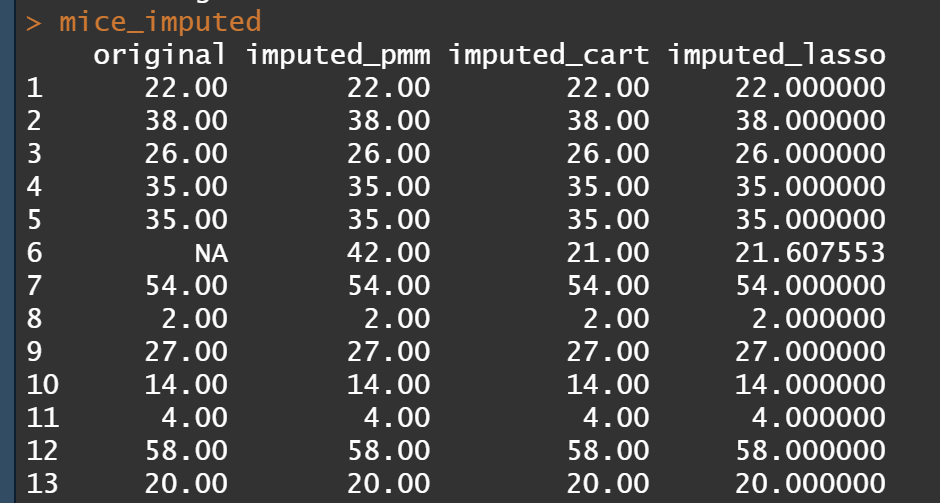
如果单从表格数据很难判断插补后对原来数据的影响,这种情况我们还是依旧做直方图进行可视化:
1h1 <- ggplot(mice_imputed, aes(x = original)) +
 2  geom_histogram(fill = "#ad1538", color = "#000000", position = "identity") +
 3  ggtitle("Original distribution") +
 4  theme_classic()
 5h2 <- ggplot(mice_imputed, aes(x = imputed_pmm)) +
 6  geom_histogram(fill = "#15ad4f", color = "#000000", position = "identity") +
 7  ggtitle("pmm-imputed distribution") +
 8  theme_classic()
 9h3 <- ggplot(mice_imputed, aes(x = imputed_cart)) +
10  geom_histogram(fill = "#1543ad", color = "#000000", position = "identity") +
11  ggtitle("cart-imputed distribution") +
12  theme_classic()
13h4 <- ggplot(mice_imputed, aes(x = imputed_lasso)) +
14  geom_histogram(fill = "#ad8415", color = "#000000", position = "identity") +
15  ggtitle("lasso-imputed distribution") +
16  theme_classic()
17plot_grid(h1, h2, h3, h4, nrow = 2, ncol = 2)
18
插补后的数据看起来更接近原始分布。但应注意的是,使用laso.norm的插补方法会使得年龄值低于零,这跟我们实际情况不一致。因此如果您选择这种插补技术,则需要手动更正负值。
3.使用 missForest 包进行插补
Miss Forest 插补技术基于随机森林算法。它是一种非参数插补方法,这意味着它不会对函数形式做出明确的假设,而是尝试以最接近数据点的方式来估计函数。
换句话说,它为每个变量建立一个随机森林模型,然后使用该模型来预测缺失值。您可以通过阅读此文章了解更多信息。
同样的,只对年龄进行插补:
1library(missForest)
2missForest_imputed <- data.frame(
3  original = titanic_numeric$Age,
4  imputed_missForest = missForest(titanic_numeric)$ximp$Age
5)
6missForest_imputed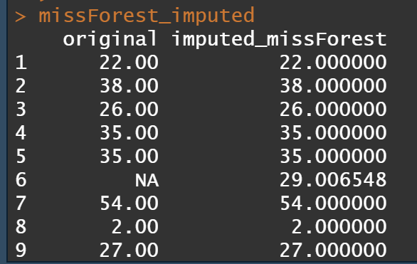
可视化插补后的数据分布与原来的数据对比:
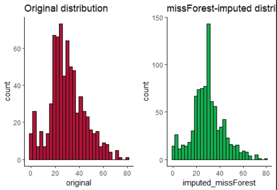
MissForest 插补后与原来的数据分布差别很大,MissForest 插补有点类似于常数值插补,因为大部分值都在 35 左右。这意味着 Miss Forest 不是我们今天看到的最好的插补技术。
小结:
掌握了以上几种常见的数据插补方法,这几种技术可用于你的数据清洗和整理过程,赶紧用起来吧。

更多实战课程
2022年以来,我们召集了一批富有经验的高校专业队伍,着手举行短期统计课程培训班,包括R语言、meta分析、临床预测模型、真实世界临床研究、问卷与量表分析、医学统计与SPSS、临床试验数据分析、重复测量资料分析、结构方程模型、孟德尔随机化等10门课。如果您有需求,不妨点击查看:
10门科研与统计课程介绍:含孟德尔随机化课程


 604
604

 被折叠的 条评论
为什么被折叠?
被折叠的 条评论
为什么被折叠?
 到【灌水乐园】发言


