


目录
4.1 在常规范围内tau是不是越大越好,像刚才的例子是不是tau取5要比4好?
1. 背景介绍
1.1 统计工具

1.2 自回归模型


1.3 马尔可夫模型

1.4 因果关系

2. 训练
在了解了上述统计工具后,让我们在实践中尝试一下! 首先,我们生成一些数据:使用正弦函数和一些可加性噪声来生成序列数据, 时间步为1,2,…,1000。
%matplotlib inline
import torch
from torch import nn
from d2l import torch as d2l

T = 1000  ''' 总共产生1000个点 '''
time = torch.arange(1, T + 1, dtype=torch.float32)
x = torch.sin(0.01 * time) + torch.normal(0, 0.2, (T,))
d2l.plot(time, [x], 'time', 'x', xlim=[1, 1000], figsize=(6, 3))
tau = 4
features = torch.zeros((T - tau, tau))
for i in range(tau):
    features[:, i] = x[i: T - tau + i]
labels = x[tau: ].reshape((-1, 1))

batch_size, n_train = 16, 600
''' 只有前n_train个样本用于训练 '''
train_iter = d2l.load_array((features[: n_train], labels[:n_train]), batch_size,
                                is_train = True)
在这里,我们使用一个相当简单的架构训练模型: 一个拥有两个全连接层的多层感知机,ReLU激活函数和平方损失。
''' 初始化网络权重的函数 '''
def init_weights(m):
    if type(m) == nn.Linear:
        nn.init.xavier_uniform_(m.weight)

''' 一个简单的多层感知机 '''
def get_net():
    net = nn.Sequential(nn.Linear(4, 10),
                        nn.ReLU(),
                        nn.Linear(10, 1))
    net.apply(init_weights)
    return net
''' 平方损失,注意MSELoss计算平方误差不带系数 1 / 2'''
loss = nn.MSELoss(reduction = 'none')
现在,准备训练模型了。实现下面的训练代码的方式与前面几节中的循环训练基本相同。因此,我们不会深入探讨太多细节。
def train(net, train_iter, loss, epochs, lr):
    trainer = torch.optim.Adam(net.parameters(), lr)
    for epoch in range(epochs):
        for X, y in train_iter:
            trainer.zero_grad()
            l = loss(net(X), y)
            l.sum().backward()
            trainer.step()
        print(f'epoch {epoch + 1}, '
              f'loss: {d2l.evaluate_loss(net, train_iter, loss):f}')

net = get_net()
train(net, train_iter, loss, 10, 0.01)
3. 预测
由于训练损失很小,因此我们期望模型能有很好的工作效果。 让我们看看这在实践中意味着什么。 首先是检查模型预测下一个时间步的能力, 也就是单步预测(one-step-ahead prediction)。
onestep_preds = net(features)
d2l.plot([time, time[tau:]],
         [x.detach().numpy(), onestep_preds.detach().numpy()],
         'time', 'x', legend = ['data', '1-step preds'],
         xlim = [1, 1000], figsize=(6, 3))

'''这里 T 代表我们最开始的自变量X的取值范围1000'''
multistep_preds = torch.zeros(T)
multistep_preds[: n_train + tau] = x[: n_train + tau]

'''从n_train + tau开始预测,每次预测使用它之前tau的时间特征值,化成(1,tau)向量训练'''
for i in range(n_train + tau, T):
    multistep_preds[i] = net(multistep_preds[i - tau: i].reshape((1, -1)))

d2l.plot([time, time[tau: ], time[n_train + tau: ]],
         [x.detach().numpy(), onestep_preds.detach().numpy(),
          multistep_preds[n_train + tau:].detach().numpy()],
         'time', 'x', legend = ['data', '1-step preds', 'multistep preds'],
         xlim=[1, 1000], figsize = (6, 3))

max_steps = 64

features = torch.zeros((T - tau - max_steps + 1, tau + max_steps))
# 列i(i<tau)是来自x的观测,其时间步从(i)到(i+T-tau-max_steps+1)
for i in range(tau):
    features[:, i] = x[i: i + T - tau - max_steps + 1]

# 列i(i>=tau)是来自(i-tau+1)步的预测,其时间步从(i)到(i+T-tau-max_steps+1)
for i in range(tau, tau + max_steps):
    features[:, i] = net(features[:, i - tau:i]).reshape(-1)

steps = (1, 4, 16, 64)
d2l.plot([time[tau + i - 1: T - max_steps + i] for i in steps],
         [features[:, (tau + i - 1)].detach().numpy() for i in steps], 'time', 'x',
         legend=[f'{i}-step preds' for i in steps], xlim=[5, 1000],
         figsize=(6, 3))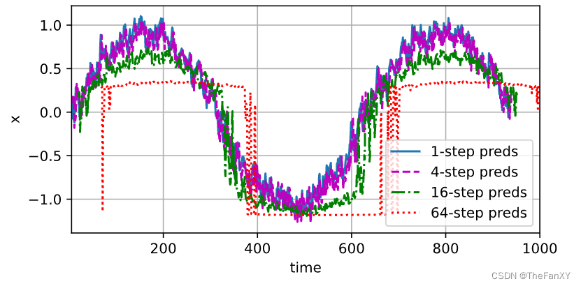
以上例子清楚地说明了当我们试图预测更远的未来时,预测的质量是如何变化的。 虽然“4步预测”看起来仍然不错,但超过这个跨度的任何预测几乎都是无用的。
4. QA
4.1 在常规范围内tau是不是越大越好,像刚才的例子是不是tau取5要比4好?
当然比4好,一般确实观察到更长更好,但是你tau大一方面样本数量少,另外一方面你特征多了,模型复杂了,其次一个时间序列越早的事物对后面的影响应该是越小,tau大了未必就一定能增加模型准确度。


 2655
2655


 被折叠的 条评论
为什么被折叠?
被折叠的 条评论
为什么被折叠?
 到【灌水乐园】发言


