Data Mining2复习笔记3 -Time Series Analysis

3. Time Series Analysis

Many “classic” DM problems have variants that respect time:
(1) frequent pattern mining → sequential pattern mining
(2) classification → predicting sequences of nominals
(3) regression → predicting the continuation of a numeric series

3.1 Sequential Pattern Mining

Finding frequent subsequences in set of sequences
the GSP algorithm

3.1.1 Application

(1) Web Usage Mining (navigation analysis)
(2) Recurring customers (allow more fine grained suggestions than frequent pattern mining - e.g. customers will select a charger after a mobile phone, but not the other way around.
(3) Using texts as a corpus (looking for common sequences of words & allows for intelligent suggestions for autocompletion)
(4) Chord progressions in music

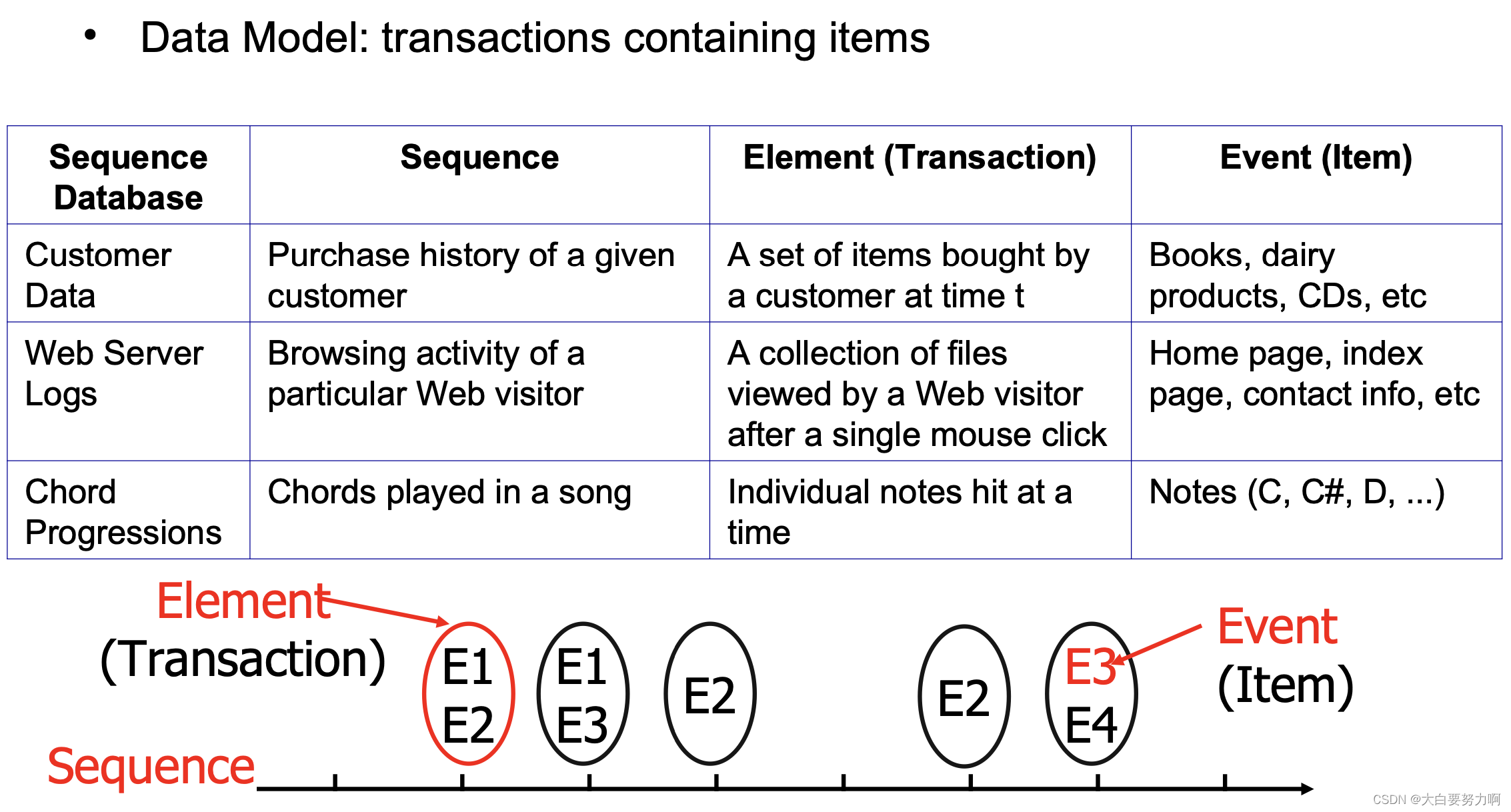
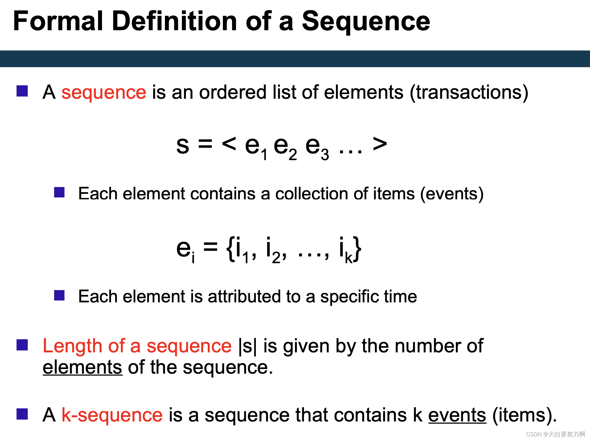
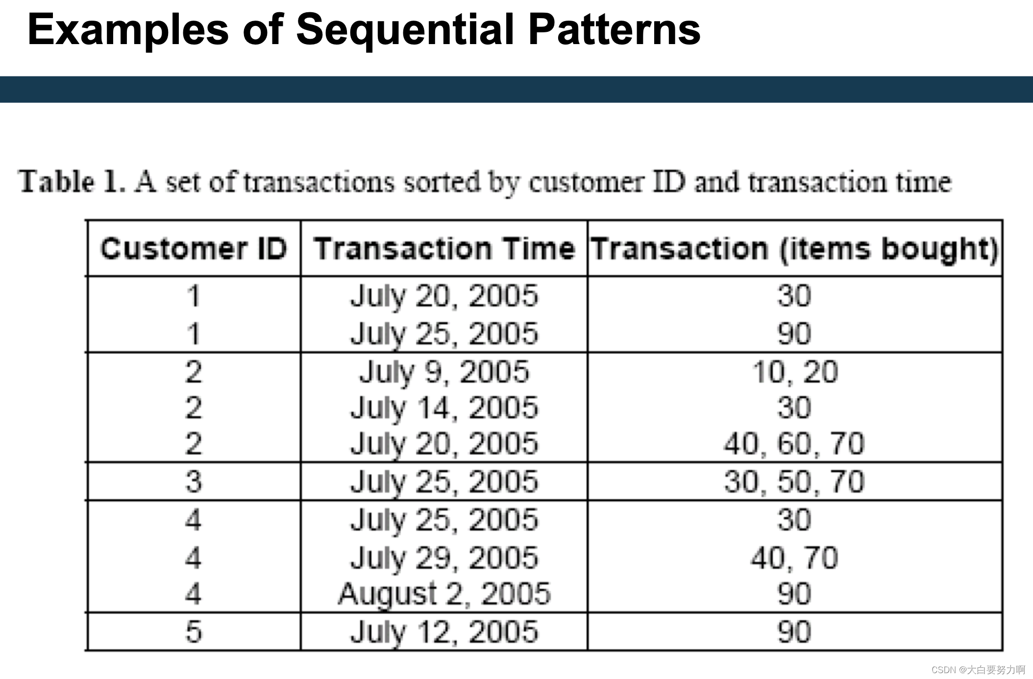
3.1.2 Sequence Data

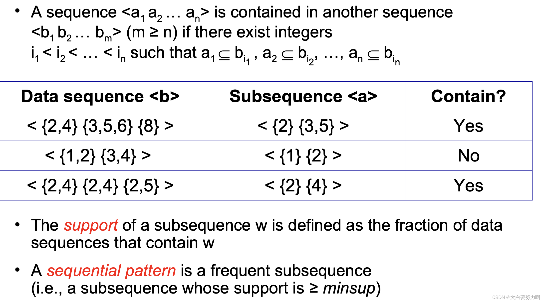
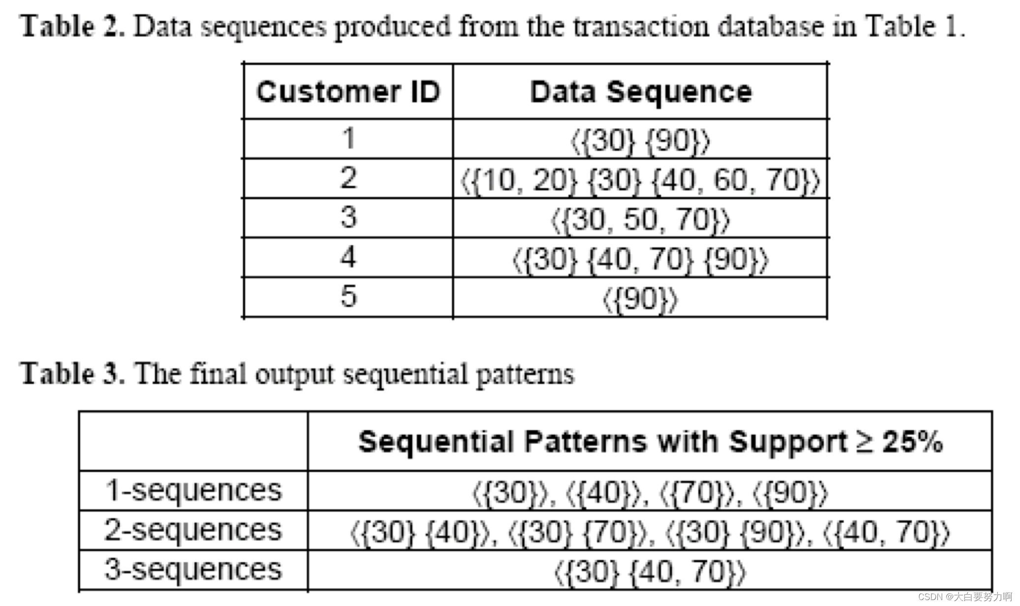
3.1.3 Sequential Pattern Mining

Given: a database of sequences and a user-specified minimum support threshold(minsup)
Task: Find all subsequences with support ≥ minsup
Challenge: Very large number of candidate subsequences (<{X},{Y}> vs.<{Y},{X}>) that need to be checked against the sequence database & By applying the Apriori principle, the number of candidates can be pruned significantly

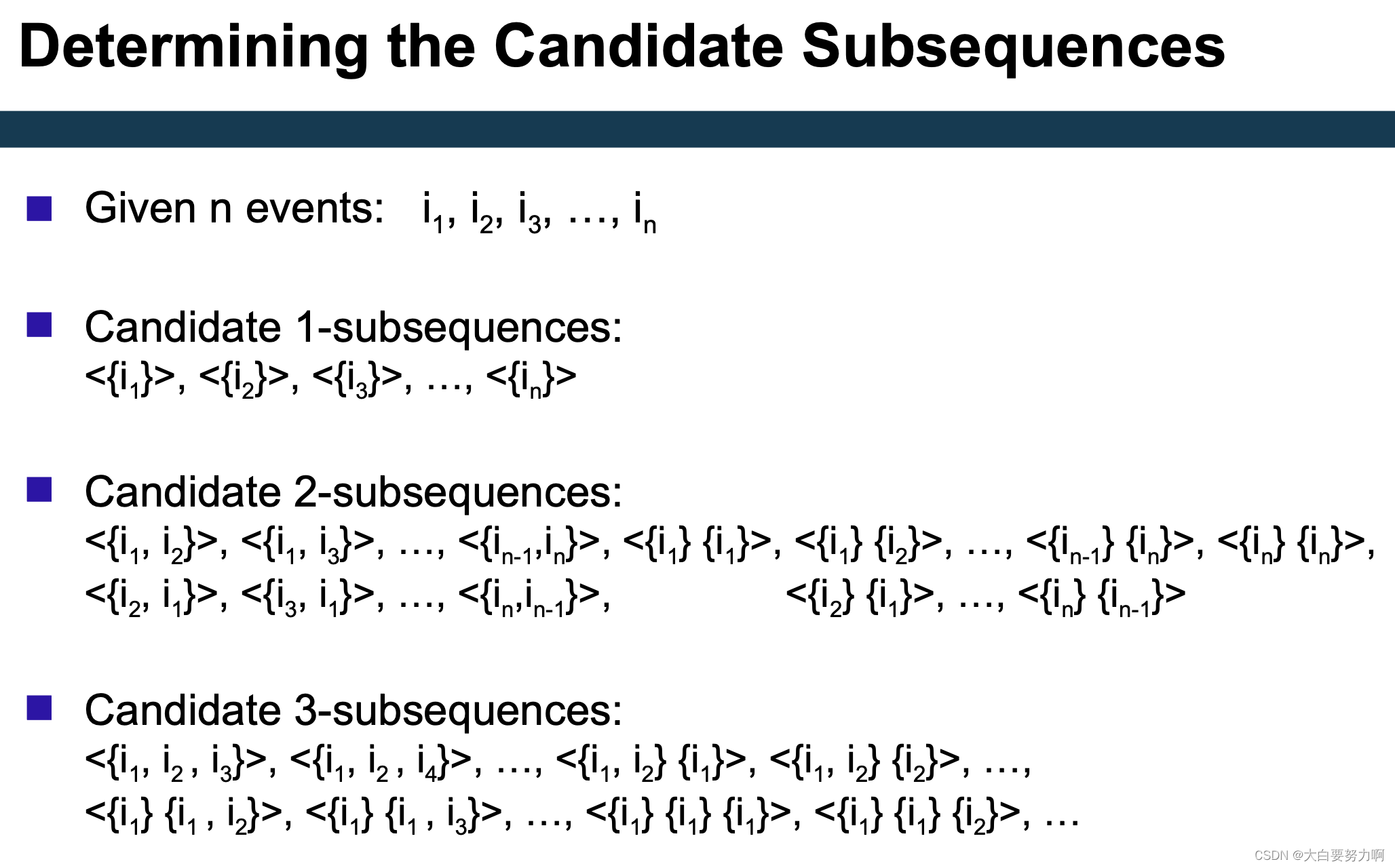
3.1.3.1 Generalized Sequencetial Pattern Algorithm (GSP)

Step 1: Make the first pass over the sequence database D to yield all the 1-element frequent subsequences

Step 2: Repeat until no new frequent subsequences are found

1. Candidate Generation
   Merge pairs of frequent subsequences found in the (k-1)th pass to generate candidate sequences that contain k items
2. Candidate Pruning
   Prune candidate k-sequences that contain infrequent (k-1)-subsequences (Apriori principle)
3. Support Counting
   Make a new pass over the sequence database D to find the support for these candidate sequences
4. Candidate Elimination
   Eliminate candidate k-sequences whose actual support is less than minsup

3.2 Trend analysis

Is a time series moving up or down?
Simple models and smoothing
Identifying seasonal effects

Task: given a time series, find out what the general trend is (e.g., rising or falling)

Possible obstacles

• random effects: ice cream sales have been low this week due to rain but what does that tell about next week?
• seasonal effects: sales have risen in December but what does that tell about January?
• cyclical effects: less people attend a lecture towards the end of the semester but what does that tell about the next semester?

3.2.1 Estimation of Trend Curves

• The freehand method
  Fit the curve by looking at the graph. Costly and barely reliable for large-scale data mining 分析人员会直接在数据图上绘制或描绘出他们认为符合趋势的曲线形状。然后，他们会尝试调整曲线，使其尽可能地拟合数据点，以获得最佳的拟合效果。
• The least-squares method
  Find the curve minimizing the sum of the squares of the deviation of points on the curve from the corresponding data points
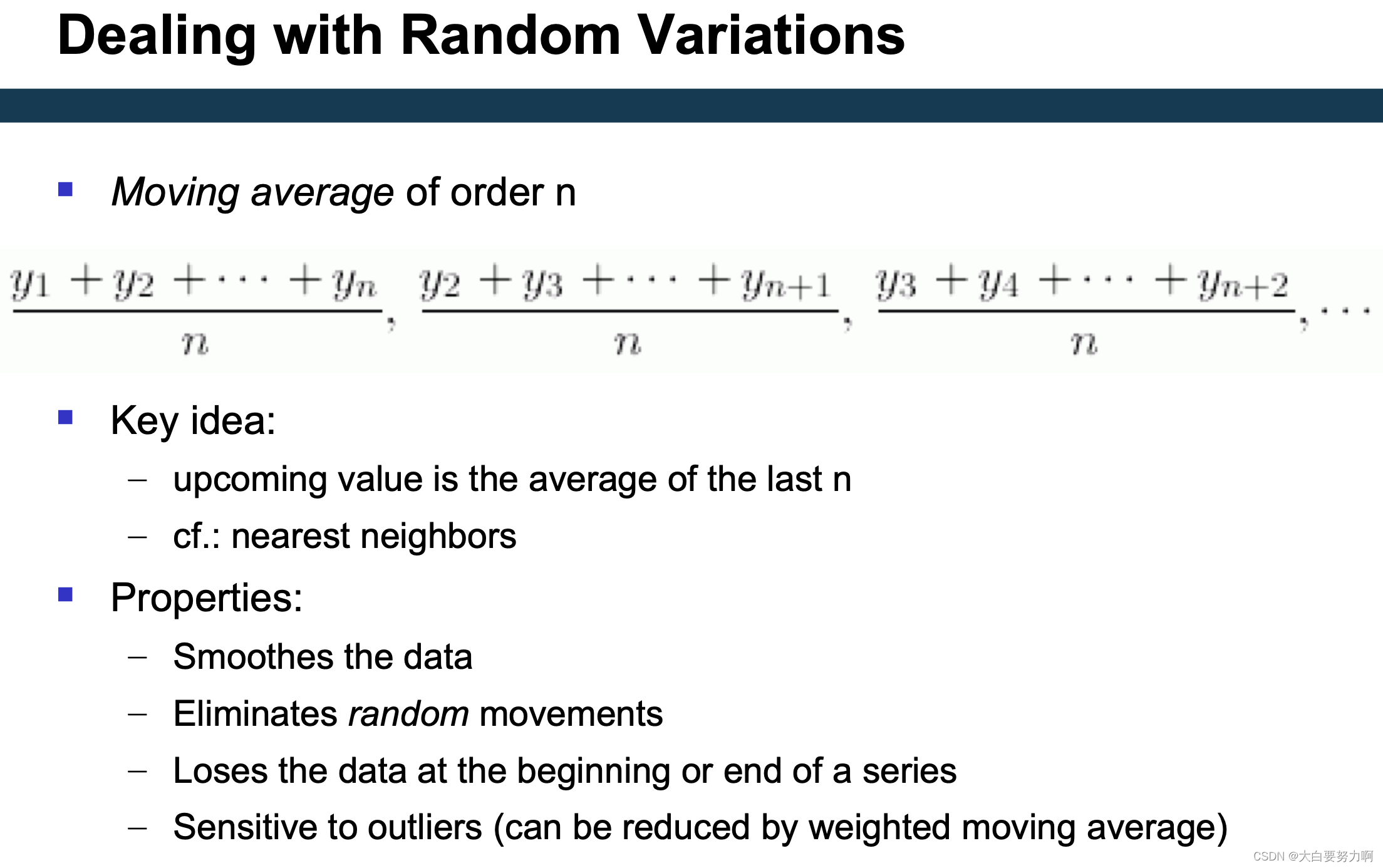
  cf. linear regression
• The moving-average method 通过计算一系列连续观测值的平均值来减少数据中的随机波动，从而显示出数据的长期趋势或周期性变化。

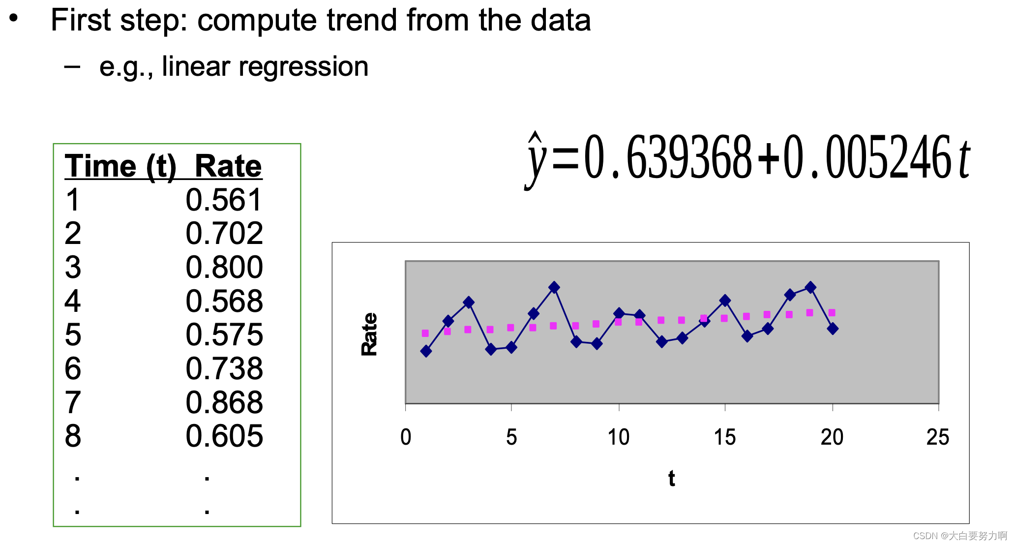
3.2.2 Linear Trend

Given a time series that has timestamps and values, i.e., (ti,vi), where ti is a time stamp, and vi is a value at that time stamp
A linear trend is a linear function: -m*ti + b
We can find via linear regression, e.g., using the least squares fit

3.2.3 A Component Model of Time Series

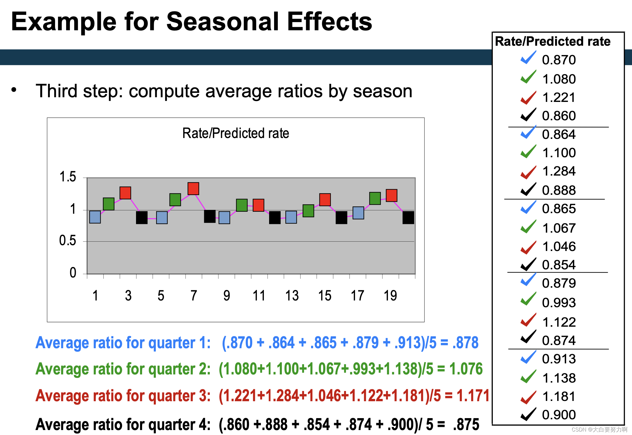
Seasonal effects occur regularly each year – quarters, months …, [Seasonal effects are repetitive upward/downward movements from the trend that occur within a calendar year at a fixed interval where periodicity is constant (e.g. every quarter, every December, every weekend, summer vs winter etc).]

Cyclical effects occur regularly over other intervals - every N years, in the beginning/end of the month, on certain weekdays or on weekends, at certain times of the day, … [Cyclical effects are fluctuations that occur around the trend line at the random interval where periodicity is not constant (e.g. holidays, business cycle, population cycles).]

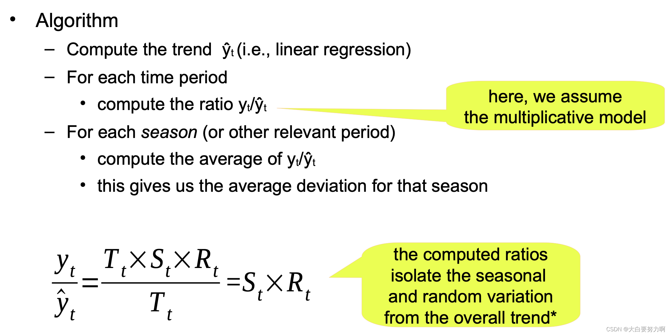
3.2.3.1 Identifying Seasonal and Cyclical Effects (periodicity is known)

here are methods of identifying and isolating those effects – given that the periodicity is known.

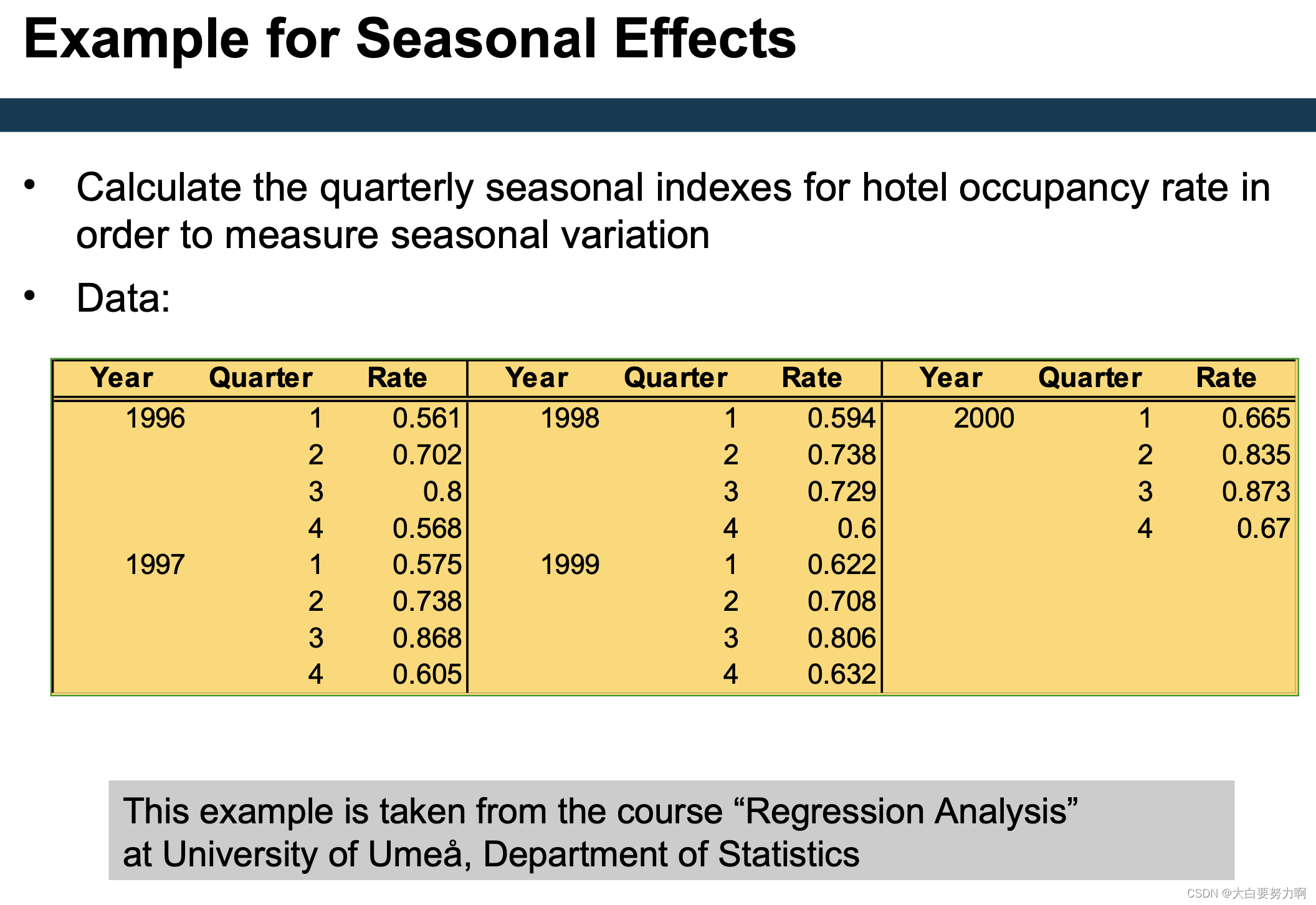
Variation may occur within a year or another period.
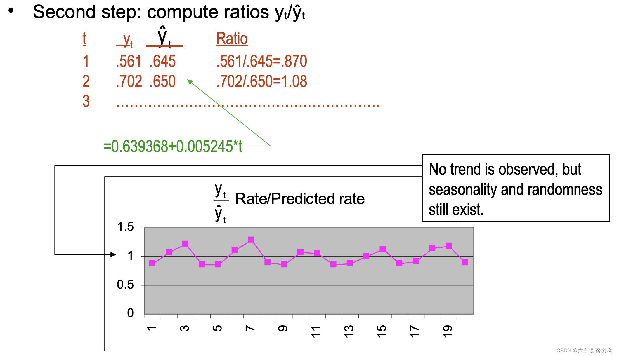
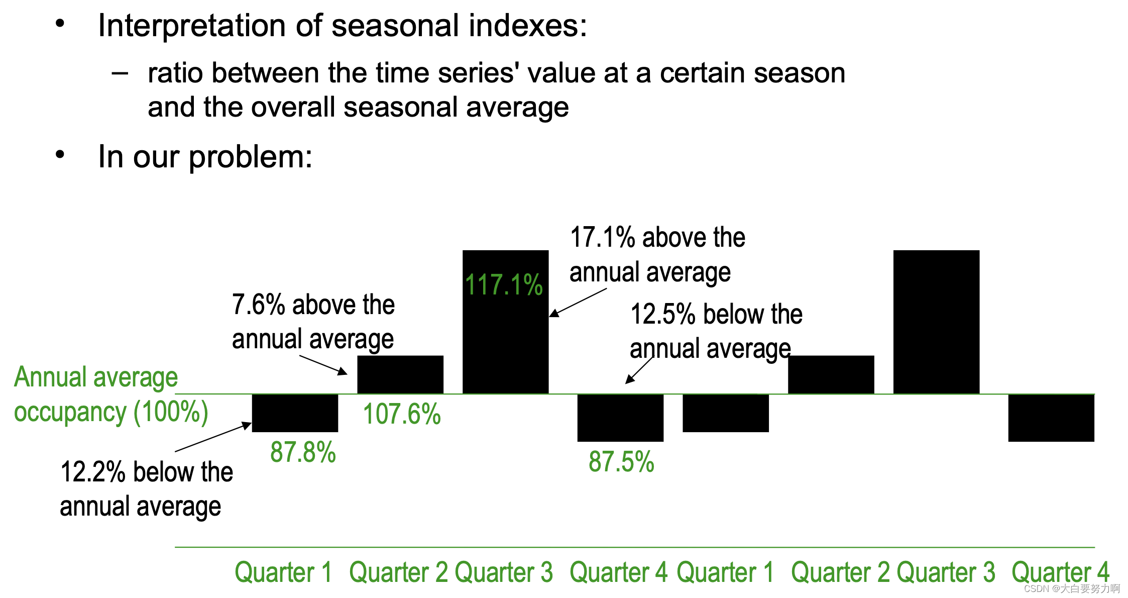
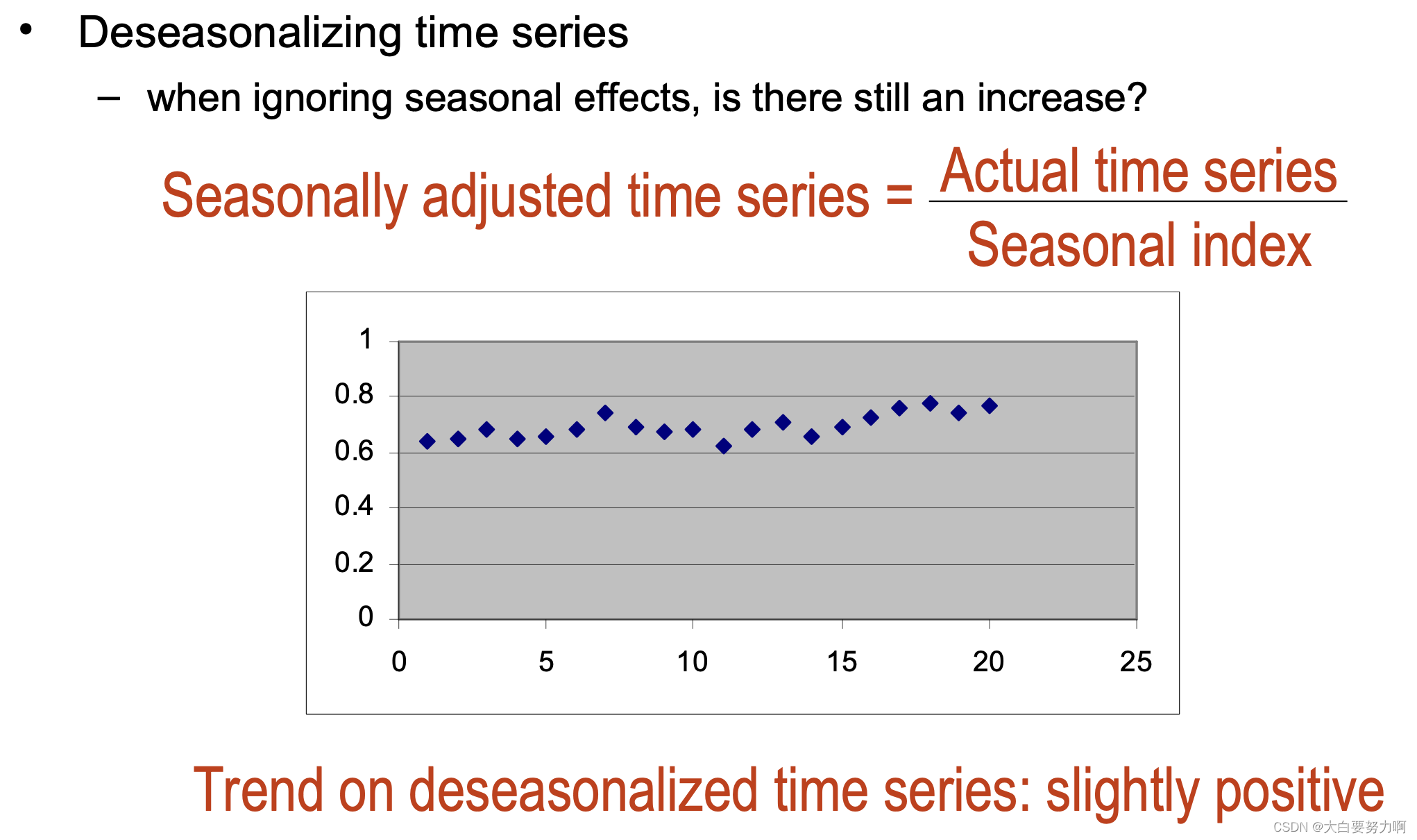
To measure the seasonal effects we compute seasonal indexes
Seasonal index: degree of variation of seasons in relation to global average 是用于衡量某一季节在相对于全年平均水平下的变动程度的指标。在时间序列分析中，季节指数用于揭示特定季节（如春季、夏季、秋季、冬季）对整体趋势的影响。

3.2.3.2 Identifying Seasonal and Cyclical Effects (periodicity is unknown)

Assumption: time series is a sum of sine waves with different periodicity and Different representation of the time series. 不同频率的正弦波之和。每个正弦波代表时间序列数据中的一个周期性效应
The frequencies of those sine waves is called spectrum
Fourier transformation transforms between spectrum and series
Spectrum gives hints at the frequency of periodic effects

Alternatives for average: median, mode, …
Often, moving averages are used for the trend
instead of a linear trend, less susceptible to outliers, the remaining computations stay the same

Recap: Trend Analysis
Allows to identify general trends (upward, downward): eliminate all other components so that only the trend remains
Method for factoring out seasonal variations and compute deseasonalized time series
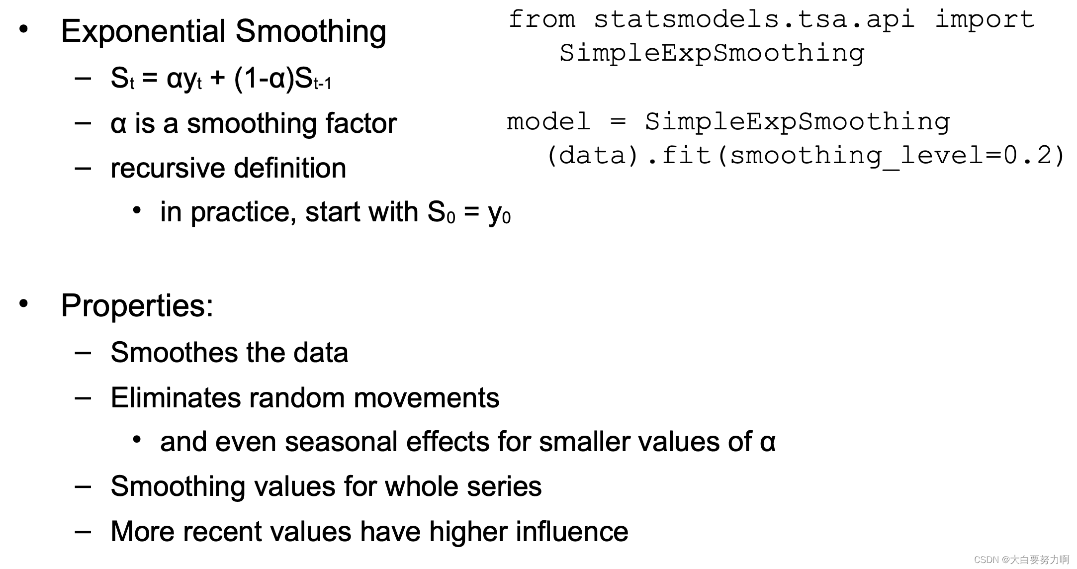
Methods for eliminating with random variations (smoothing): moving average & exponential smoothing

3.3 Forecasting

Predicting future developments from the past
Autoregressive models and windowing
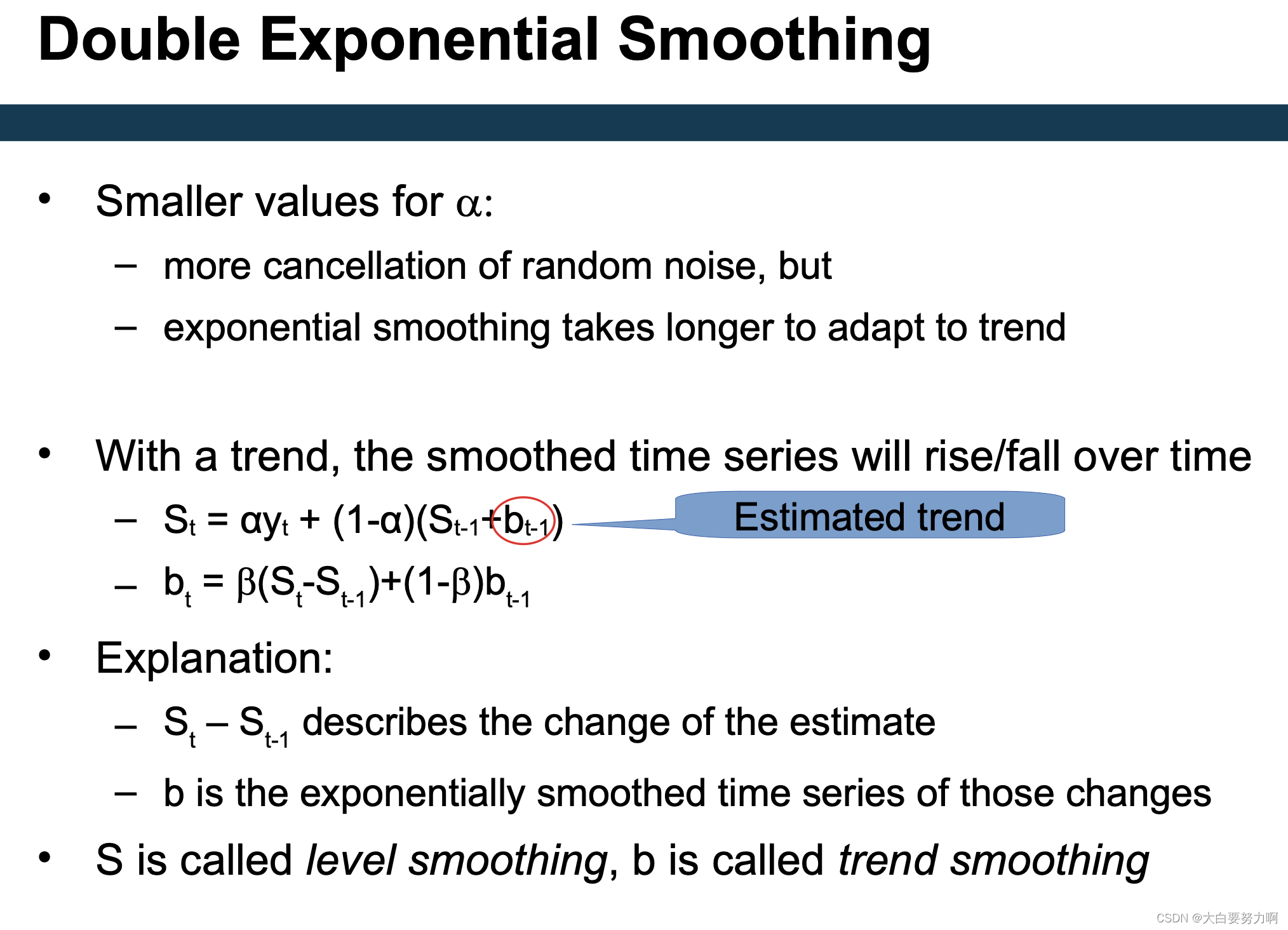
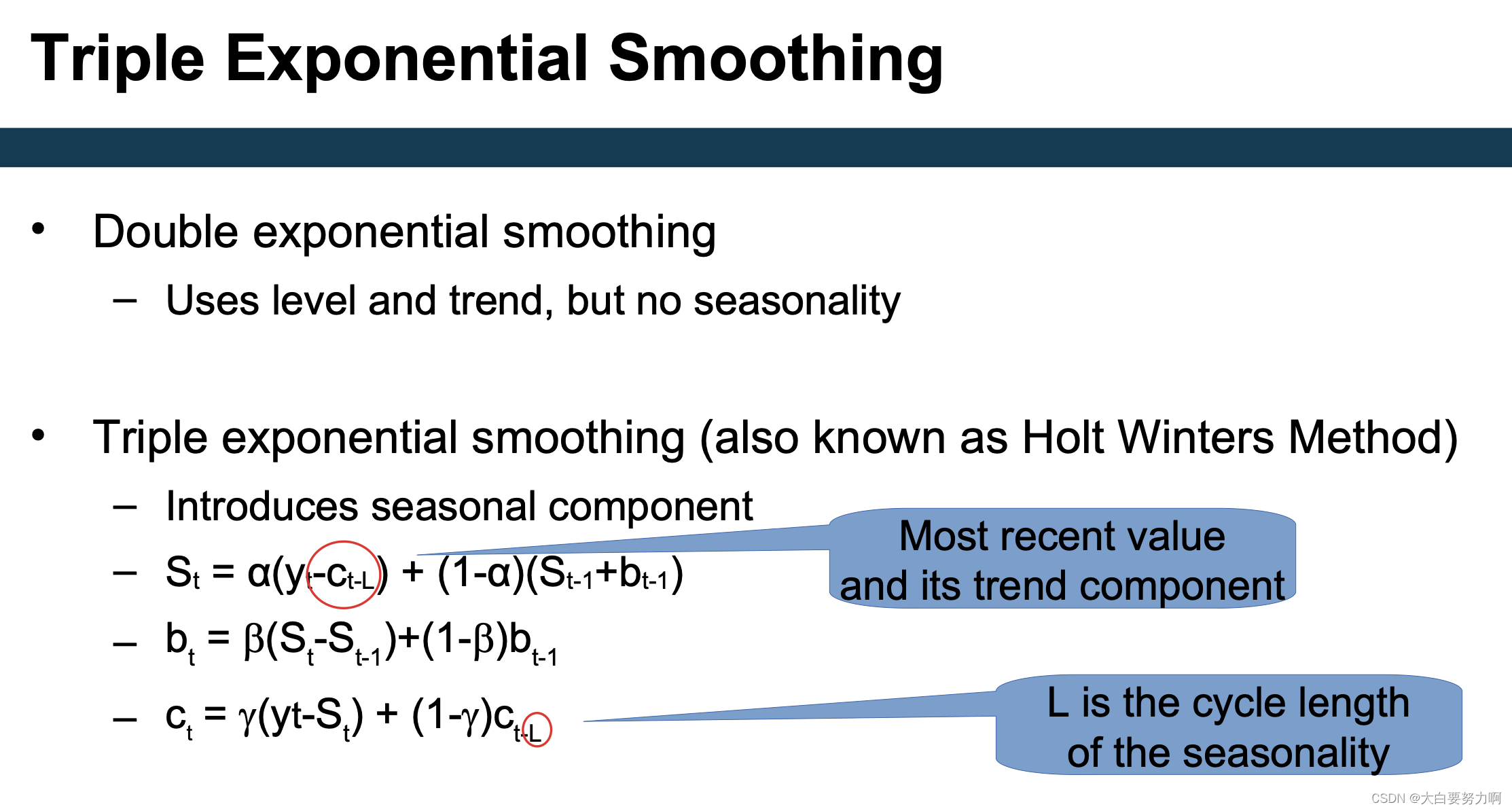
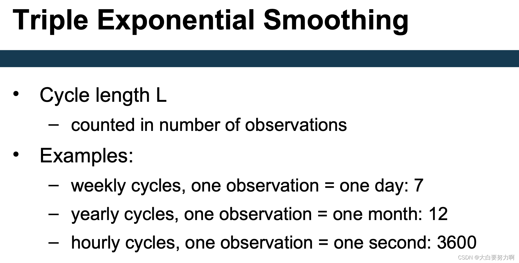
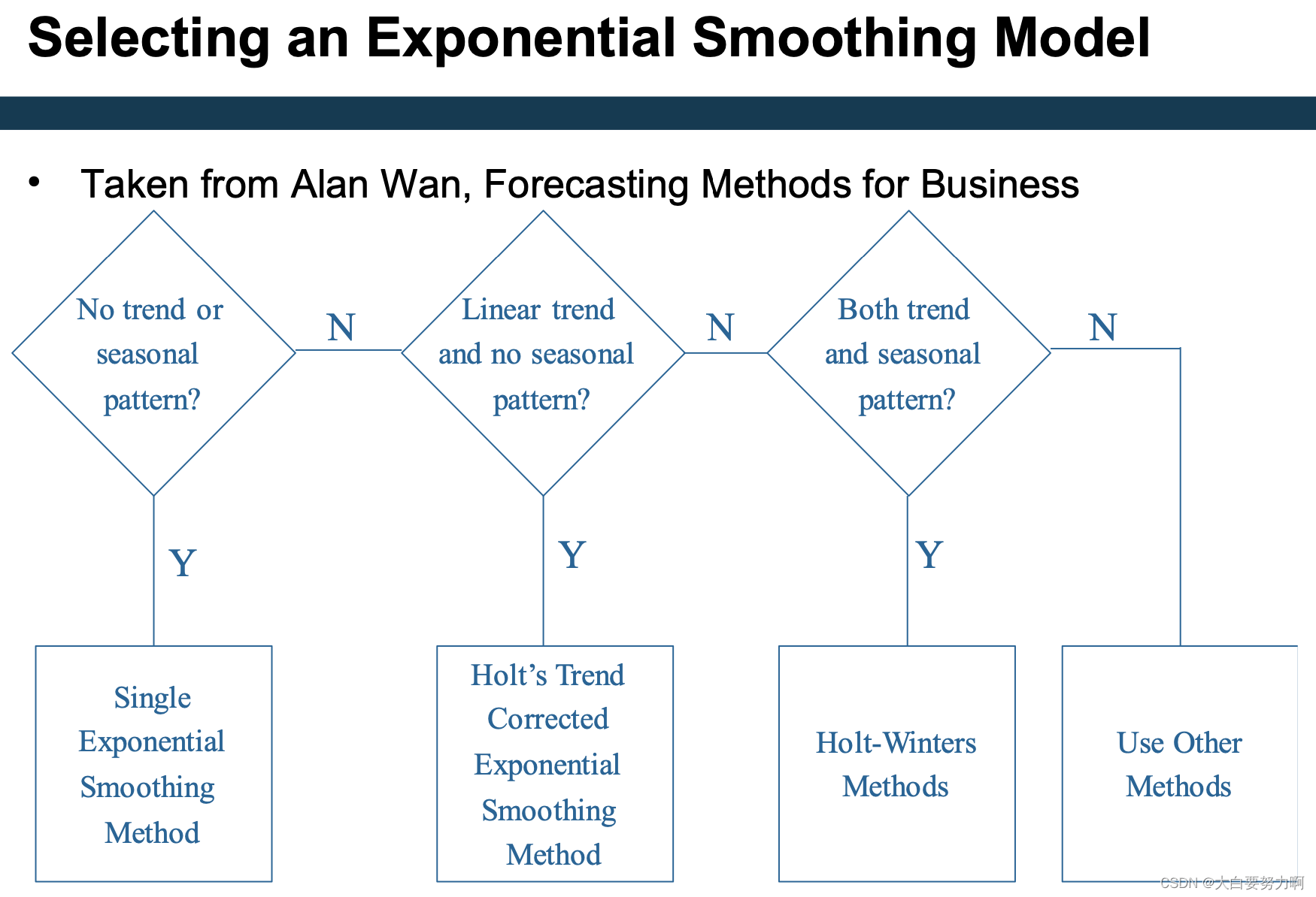
Exponential smoothing and its extensions

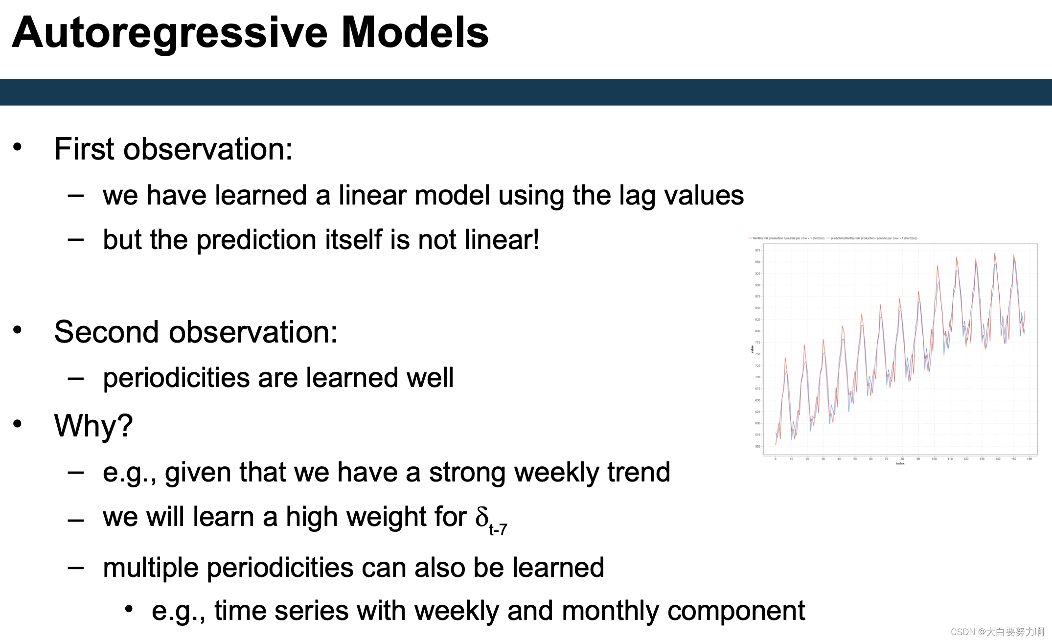
3.3.1 Autoregressive Models

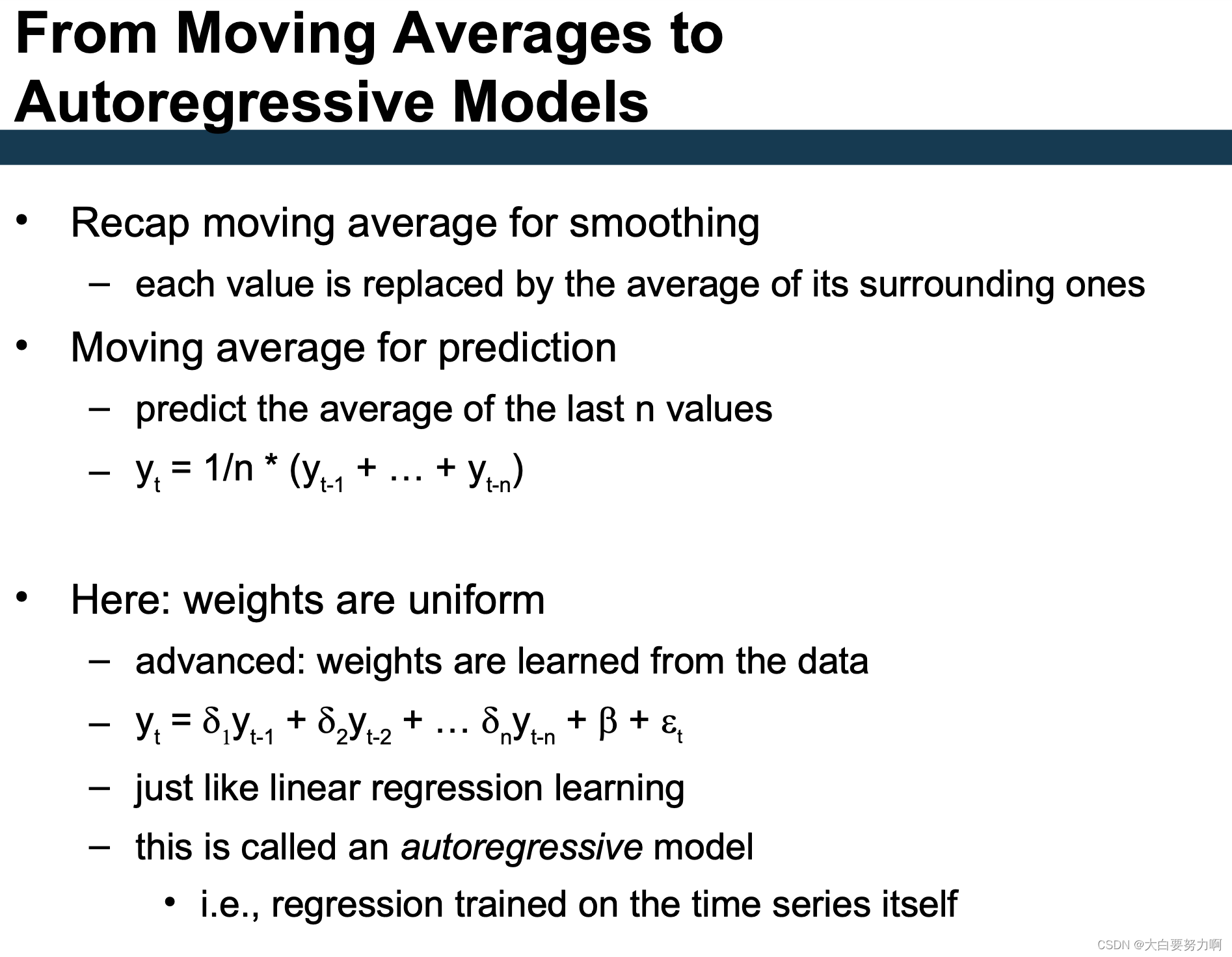
Manual approach: generate windowed representation for learning first and learn linear model on top

3.3.2 Extension of AR models

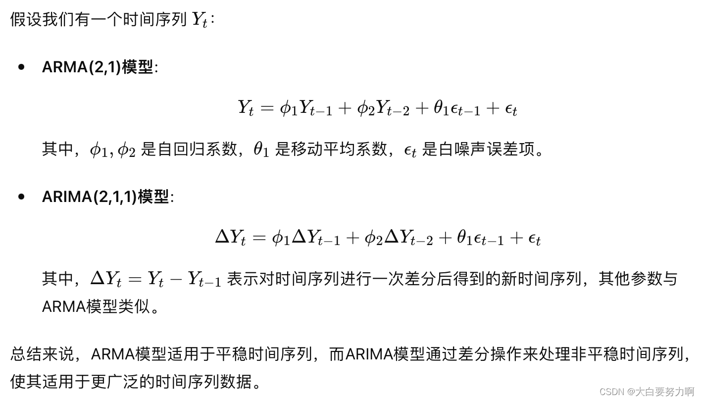
ARMA: Autoregressive Moving Average Model
ARIMA: Autoregressive Integrated Moving Average Model

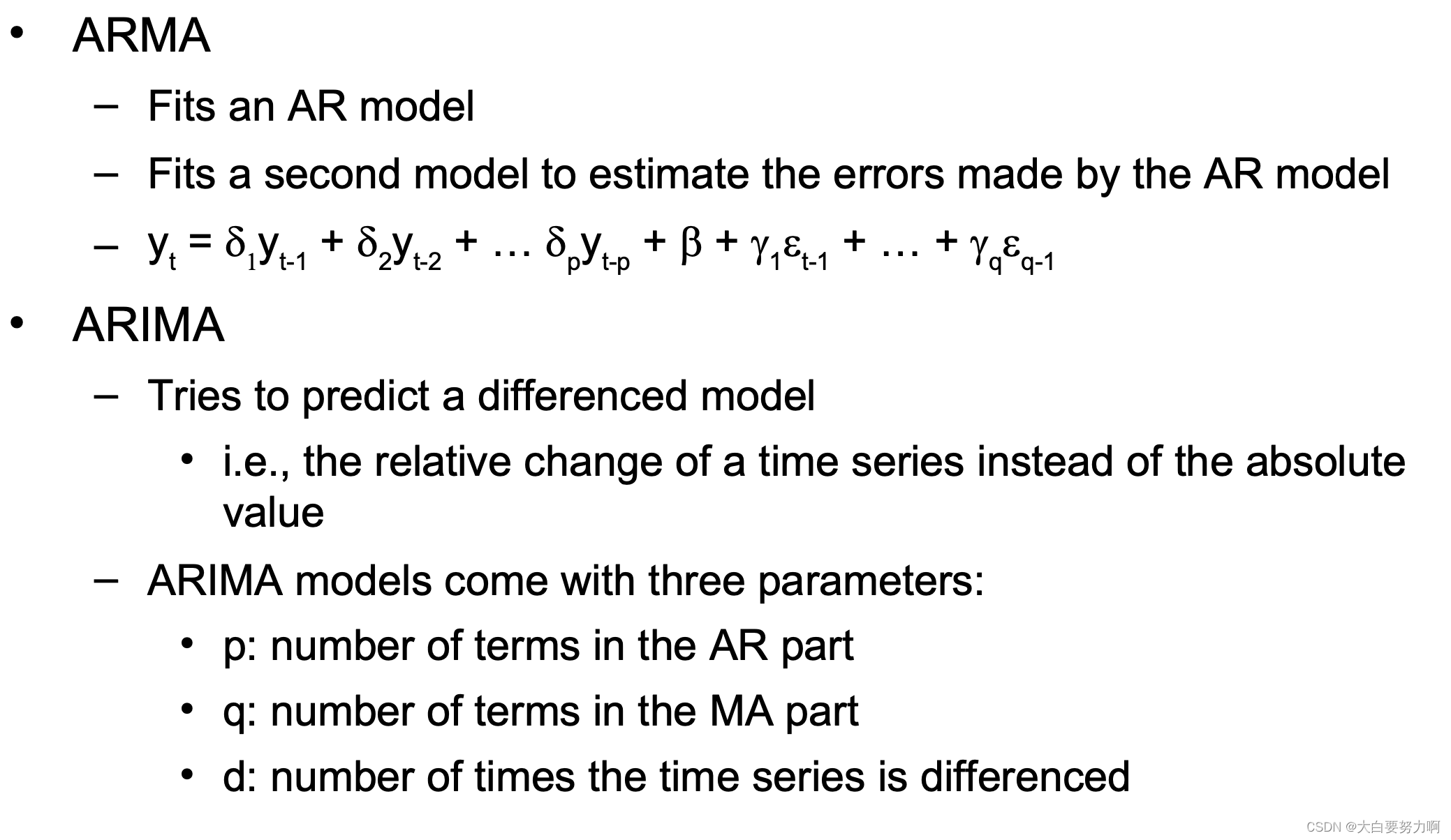
p: AR part自回归部分-当前观测值与过去观测值之间的关系，用过去p个观测值的线性组合来预测当前观测值，p是自回归阶数
q: MA part移动平均部分-当前观测值与过去预测误差之间的关系，用过去q个预测误差的线性组合来预测当前的观测值，q是移动平均阶数
d：difference差分-对时间序列数据进行减法运算，从而使数据变得平稳。平稳的时间序列的特点是均值和方差在时间上保持不变。

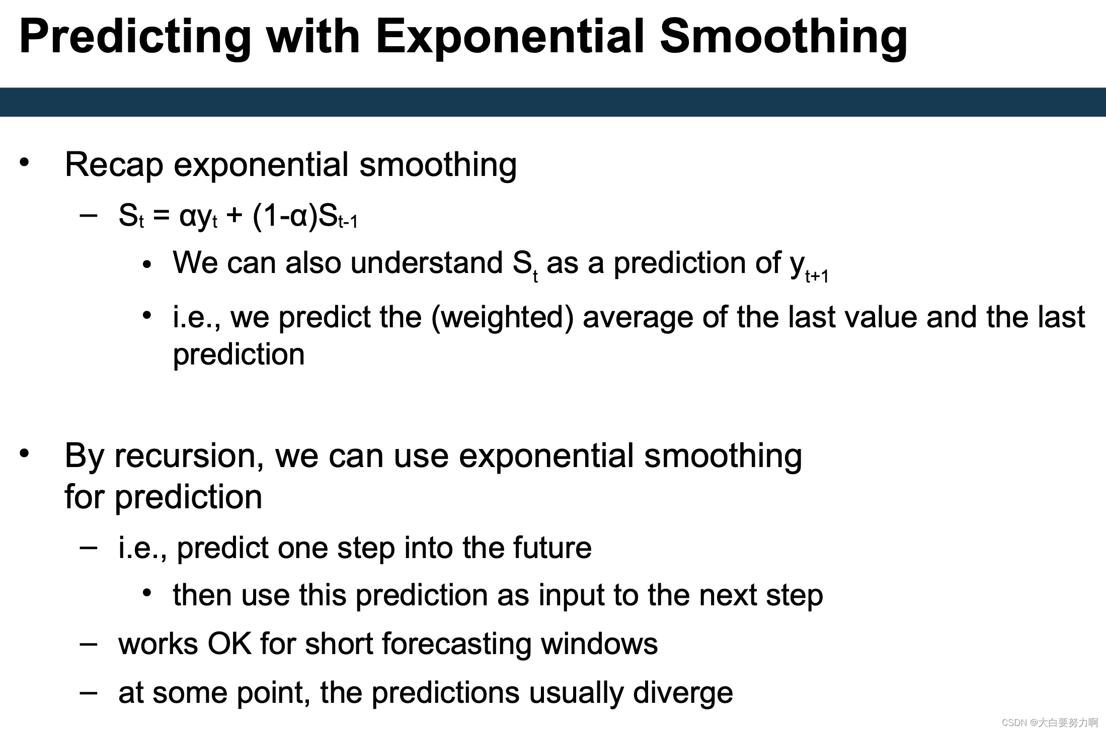
3.3.3 Predicting with Exponential Smoothing

3.3.4 Missing Values in Series Data

Remedies in non-series data

• replace with average, median, most frequent – Imputation(e.g.,k-NN)
• replace with most frequent
• …

In time series:

• Replace with average
• Linear interpolation
• Replace with previous
• Replace with next
• K-NN imputation (Essentially: this is the average of previous and next)

3.3.5 Evaluating Time Series Prediction

Cross Validation
Variant 1: Use hold out set at the end of the training data
– E.g., train on 2000-2015, evaluate on 2016

Variant 2: Sliding window evaluation
– E.g., train on one year, evaluate on consecutive year

3.4 Summary