PyTorch深度学习实践 Lecture05 线性回归

🤵 Author ：Horizon John

✨ 编程技巧篇：各种操作小结

🎇 机器视觉篇：会变魔术 OpenCV

💥 深度学习篇：简单入门 PyTorch

🏆 神经网络篇：经典网络模型

💻 算法篇：再忙也别忘了 LeetCode

视频链接：Lecture 05 Linear_Regression_with_PyTorch
文档资料：

//Here is the link:
课件链接：https://pan.baidu.com/s/1vZ27gKp8Pl-qICn_p2PaSw
提取码：cxe4

Linear_Regression_with_PyTorch（使用PyTorch实现线性回归）

概述

PyTorch Fashion

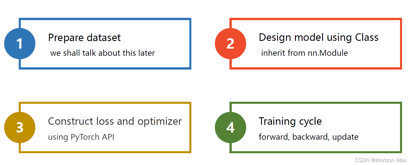
利用PyTorch建模的 基本流程 ：

1、Prepare dataset

2、Design model using Class

3、Construct loss and optimizer

4、Training cycle

下面结合代码概述以上 基本流程 ：

Code

# Here is the code :

import torch

# 1、Prepare dataset

x_data = torch.tensor([[1.0], [2.0], [3.0]])
y_data = torch.tensor([[2.0], [4.0], [6.0]])
 
 
# 2、Design model using Class

class LinearModel(torch.nn.Module):   # Our model class should be inherit from nn.Module
                                      # which is Base class for all neural network modules
    def __init__(self):
        super(LinearModel, self).__init__()
        self.linear = torch.nn.Linear(1, 1)   # nn.Linear(1, 1)输入输出维度均为1
 
    def forward(self, x):  # 前向传播
        y_pred = self.linear(x)
        return y_pred  
 
model = LinearModel()

 
# 3、Construct loss and optimizer

criterion = torch.nn.MSELoss(reduction = 'sum')   # 即返回loss.sum()，默认 reduction='mean' 返回 loss.mean()
optimizer = torch.optim.SGD(model.parameters(), lr = 0.01)   # model.parameters()参数初始化
 
 
# 4、Training cycle

for epoch in range(100):
    y_pred = model(x_data)               # forward（得到预测值 y_hat）
    loss = criterion(y_pred, y_data)     # 计算loss值
    print(epoch, loss.item())
 
    optimizer.zero_grad()  # grad 参数置零
    loss.backward()        # backward（会自动计算梯度）
    optimizer.step()       # update（更新参数 w 和 b）
 
print('w = ', model.linear.weight.item())
print('b = ', model.linear.bias.item())
 
x_test = torch.tensor([[4.0]])     # 预测 x=4 时 y 的值
y_test = model(x_test)
print('y_pred = ', y_test.data)

运行结果

0 50.871299743652344
1 23.290237426757812
2 11.00268268585205
3 5.523491859436035
4 3.0753233432769775
5 1.9766101837158203
      ... ...
96 0.29678839445114136
97 0.29252320528030396
98 0.2883186936378479
99 0.2841755151748657

w =  1.6451170444488525
b =  0.8067324757575989
y_pred =  tensor([[7.3872]])

Exercise

选择不同的优化器（Optimizer）查看网络运行效果

Code

# Here is the code :

import torch
import matplotlib.pyplot as plt


# 1、Prepare dataset

x_data = torch.tensor([[1.0], [2.0], [3.0]])
y_data = torch.tensor([[2.0], [4.0], [6.0]])


# 2、Design model using Class

class LinearModel(torch.nn.Module):  # Our model class should be inherit from nn.Module
    # which is Base class for all neural network modules
    def __init__(self):
        super(LinearModel, self).__init__()
        self.linear = torch.nn.Linear(1, 1)  # nn.Linear(1, 1)输入输出维度均为1

    def forward(self, x):  # 前向传播
        y_pred = self.linear(x)
        return y_pred


model = LinearModel()


# 3、Construct loss and optimizer

criterion = torch.nn.MSELoss(reduction='sum')
optimizer = torch.optim.SGD(model.parameters(), lr=0.01)  # model.parameters()参数初始化


# 4、Training cycle

epoch_list = []  # 构建数组存放迭代过程中的 epoch 和 cost 值
cost_list = []

for epoch in range(100):
    y_pred = model(x_data)  # forward（得到预测值 y_hat）
    loss = criterion(y_pred, y_data)  # 计算loss值

    epoch_list.append(epoch)
    cost_list.append(loss.item()/len(x_data))

    optimizer.zero_grad()  # grad 参数置零
    loss.backward()  # backward（会自动计算梯度）
    optimizer.step()  # update（更新参数 w 和 b）

print('w = ', model.linear.weight.item())
print('b = ', model.linear.bias.item())

x_test = torch.tensor([[4.0]])  # 预测 x=4 时 y 的值
y_test = model(x_test)
print('y_pred = ', y_test.data)

plt.plot(epoch_list, cost_list)  # 绘图
plt.title('SGD')
plt.xlabel('Epoch')
plt.ylabel('cost')
plt.show()

神经网络优劣的指标—— 代价函数（Cost Function）

我们需要通过 优化器（Optimizer） 不断改进神经网络来使 代价函数 最小

八种优化器比较（optimizer）

各优化器介绍参考 Pytorch中文文档

torch.optim.Adagrad()

def __init__(self, params, lr=1e-2, lr_decay=0, weight_decay=0, initial_accumulator_value=0, eps=1e-10):

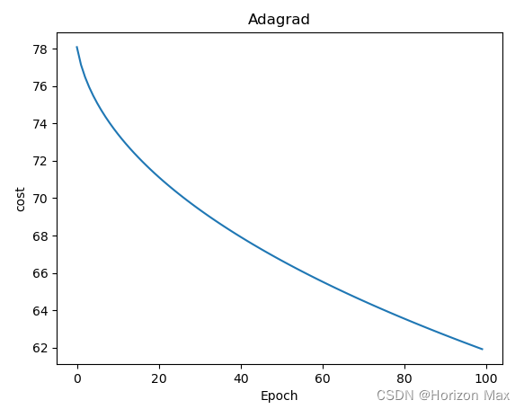
w =  -0.0708811953663826
b =  -0.07163553684949875
y_pred =  tensor([[-0.3552]])

torch.optim.Adam()

def __init__(self, params, lr=1e-3, betas=(0.9, 0.999), eps=1e-8,
                 weight_decay=0, amsgrad=False):

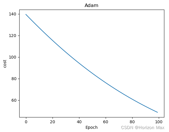
w =  0.051138054579496384
b =  0.2211645096540451
y_pred =  tensor([[0.4257]])

torch.optim.Adamax()

def __init__(self, params, lr=2e-3, betas=(0.9, 0.999), eps=1e-8,
                 weight_decay=0):

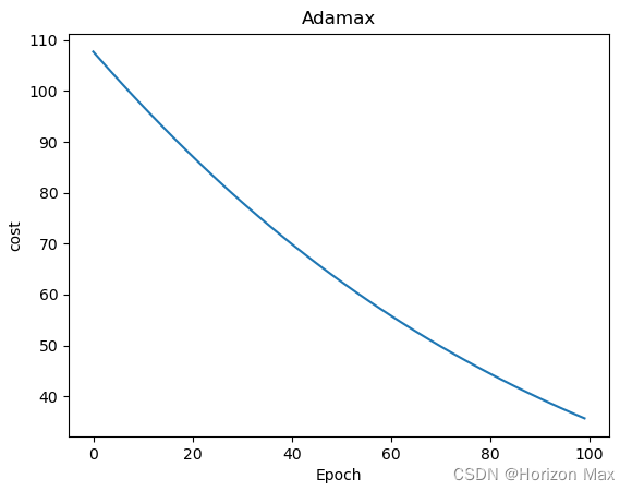
w =  -0.0033778981305658817
b =  0.9950549006462097
y_pred =  tensor([[0.9815]])

torch.optim.ASGD()

def __init__(self, params, lr=1e-2, lambd=1e-4, alpha=0.75, t0=1e6, weight_decay=0)：

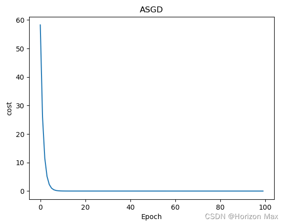
w =  2.03299617767334
b =  -0.07502224296331406
y_pred =  tensor([[8.0570]])

torch.optim.LBFGS()

def __init__(self,
                 params,
                 lr=1,    # 学习率 默认1
                 max_iter=20,     # (int) 最大迭代次数 默认20
                 max_eval=None,      # (int) 最大函数评价次数 默认max_iter * 1.25
                 tolerance_grad=1e-7,     # (float) 一阶最优的终止容忍度 默认1e-5
                 tolerance_change=1e-9,     # (float) 函数值/参数变化量的终止容忍度 默认1e-9
                 history_size=100,      # (int) 更新历史的大小 默认100
                 line_search_fn=None):

一些优化算法 例如 Conjugate Gradient 和 LBFGS 需要重复多次计算函数

因此需要传入一个闭包去允许它们重新计算你的模型，这个闭包会清空梯度， 计算损失，然后返回。

代码如下：

for epoch in range(100):
    def closure():
        y_pred = model(x_data)  # forward（得到预测值 y_hat）
        loss = criterion(y_pred, y_data)  # 计算loss值

        epoch_list.append(epoch)
        cost_list.append(loss.item()/len(x_data))

        optimizer.zero_grad()  # grad 参数置零
        loss.backward()  # backward（会自动计算梯度）
        return loss

    optimizer.step(closure)  # update（更新参数 w 和 b）

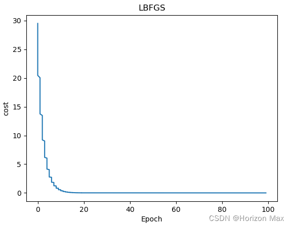
w =  1.999942421913147
b =  4.552656173473224e-05
y_pred =  tensor([[7.9998]])

torch.optim.RMSprop()

def __init__(self, params, lr=1e-2, alpha=0.99, eps=1e-8, weight_decay=0, momentum=0, centered=False):

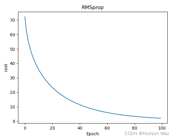
w =  1.115038275718689
b =  1.3704285621643066
y_pred =  tensor([[5.8306]])

torch.optim.Rprop()

def __init__(self, params, lr=1e-2, etas=(0.5, 1.2), step_sizes=(1e-6, 50)):

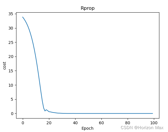
w =  1.9998326301574707
b =  0.00040745444130152464
y_pred =  tensor([[7.9997]])

torch.optim.SGD()

def __init__(self, params, lr=required, momentum=0, dampening=0,
                 weight_decay=0, nesterov=False):

w =  1.662644386291504
b =  0.7668885588645935
y_pred =  tensor([[7.4175]])

参考：https://ruder.io/optimizing-gradient-descent/index.html

附录：相关文档资料

PyTorch 官方文档： PyTorch Documentation
PyTorch 中文手册： PyTorch Handbook

《PyTorch深度学习实践》系列链接：

  Lecture01 Overview
  Lecture02 Linear_Model
  Lecture03 Gradient_Descent
  Lecture04 Back_Propagation
  Lecture05 Linear_Regression_with_PyTorch
  Lecture06 Logistic_Regression
  Lecture07 Multiple_Dimension_Input
  Lecture08 Dataset_and_Dataloader
  Lecture09 Softmax_Classifier
  Lecture10 Basic_CNN
  Lecture11 Advanced_CNN
  Lecture12 Basic_RNN
  Lecture13 RNN_Classifier