感知机与BP神经网络

一、感知机

1.1感知机模型

感知机是一种线性二分类模型，对直线的两侧分类，当wx+b>0时为1，当wx+b<0时为-1。
$$f(x)=sign(x)=\{\begin{array}{ll}1,& \text{x>0}\\ -1,& \text{x<0}\end{array}$$
$$y=f(w\cdot x+b)$$

1.2损失函数

$$L(w,b)=-\sum _{x_i\in M}{y}_i\cdot (w\cdot x_i+b)$$
其中w为权重，b为偏置，M是误分类点的集合
M = { x i ∣ y i ( w ⋅ x i + b ) < = 0 } M=\{x_i|y_i(w\cdot x_i+b)<=0\} M={xi​∣yi​(w⋅xi​+b)<=0}
求损失函数的最小值，不断调整w、b的值
使损失函数最小：
$$minL(w,b)=-\sum _{x_i\in M}{y}_i(w\cdot x_i+b)$$
损失函数的梯度为：
$${▽}_{w}L(w,b)=-\sum _{x_i\in M}{y}_i{x}_i$$

$${▽}_{b}L(w,b)=-\sum _{x_i\in M}{y}_i$$
w、b更新为：
$$w=w+\eta \sum _{x_i\in M}{y}_i{x}_i$$
$$b=b+\eta \sum _{x_i\in M}{y}_i$$

1.3算法

输入：训练数据 T = { ( x 1 , y 1 ) , ( x 2 , y 2 ) . . . . ( x n , y n ) } ， 学 习 率 η T=\{(x_1,y_1),(x_2,y_2)....(x_n,y_n)\}，学习率η T={(x1​,y1​),(x2​,y2​)....(xn​,yn​)}，学习率η
输出：w、b
1.对w、b进行初始化
2.选取训练数据$(x_i,y_i)$
3.判断该点是否为误分类点，如果$y_i(w{x}_i+b)<=0)$,则：
   $w=w+\eta y_i{x}_i$
   $b=b+\eta y_i$
4.转到步骤2，直到训练数据集中没有误分类点

二、BP神经网络

2.1基本思想

BP神经网络是一种后向传播学习的前馈型神经网络。BP神经网络模型拓扑结构包括输入层（input）、隐层(hide layer)和输出层(output layer)。
BPNN的前馈型神经网络是一种结构，指在处理样本的时候，从输入层输入，向前把结果输出到第一隐含层，然后第一隐含层将接受的数据处理后作为输出，该输出作为第二隐含层的输入，以此类推，直到输出层的输出为止。
反向传播是一种学习算法，通过比较输出层的实际输出和预期的结果，得到误差，然后通过相关的误差方程式调整最后一个隐含层到输出层之间的网络权重，之后从最后一个隐含层向倒数第二隐含层进行误差反馈，调整他们之间的网络权重，以此类推，直到输入层与第一隐含层之间的网络权重调整为止。

BP神经网络结构如下：

2.2前馈过程

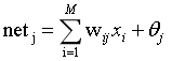
设网络输入为x，则隐含层第j个节点的输入为：

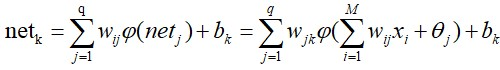
网络输出层第k个节点的输入为：

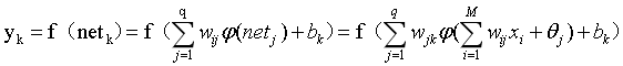
因此，网络输出层第k个节点的输出为：

2.3 算法

输入：网络结构参数（层数、节点数），训练数据集
输出：网络权值与阈值
1.网络权值初始化
2.对输入训练 S = { ( x 1 , t 1 ) , ( x 2 , t 2 ) . . . . ( x k , t k ) } S=\{(x_1,t_1),(x_2,t_2)....(x_k,t_k)\} S={(x1​,t1​),(x2​,t2​)....(xk​,tk​)}，依次通过输入层，隐含层，输出层，并分别计算误差。
3.通过误差$E$反传计算每个神经元的误差信号
4.根据误差信号调整网络权值$W$和节点阈值$\theta$
5.对训练数据不断滚动，直至最大滚动次数或误差低于某一阈值为止。

三、实现代码

感知器部分

% 第一章  感知器
% 1. 感知器神经网络的构建
% 1.1  生成网络
net=newp([0 2],1);%单输入，输入值为[0,2]之间的数
inputweights=net.inputweights{1,1};%第一层的权重为1
biases=net.biases{1};%阈值为1
% 1.2  网络仿真

net=newp([-2 2;-2 2],1);%两个输入，一个神经元，默认二值激活
net.IW{1,1}=[-1 1];%权重，net.IW{i,j}表示第i层网络第j个神经元的权重向量
net.IW{1,1}
net.b{1}=1;
net.b{1}
p1=[1;1],a1=sim(net,p1)
p2=[1;-1],a2=sim(net,p2)
p3={[1;1] [1 ;-1]},a3=sim(net,p3) %两组数据放一起
p4=[1 1;1 -1],a4=sim(net,p4)%也可以放在矩阵里面
net.IW{1,1}=[3,4];
net.b{1}=[1];
a1=sim(net,p1)
% 1.3  网络初始化
net=init(net);
wts=net.IW{1,1}
bias=net.b{1}
% 改变权值和阈值为随机数
net.inputweights{1,1}.initFcn='rands';
net.biases{1}.initFcn='rands';
net=init(net);
bias=net.b{1}
wts=net.IW{1,1}
a1=sim(net,p1)

% 2. 感知器神经网络的学习和训练
% 1 网络学习
net=newp([-2 2;-2 2],1);
net.b{1}=[0];
w=[1 -0.8]
net.IW{1,1}=w;
p=[1;2];
t=[1];
a=sim(net,p)
e=t-a
help learnp
dw=learnp(w,p,[],[],[],[],e,[],[],[],[],[])
w=w+dw
net.IW{1,1}=w;
a=sim(net,p)


net = newp([0 1; -2 2],1);
P = [0 0 1 1; 0 1 0 1];
T = [0 1 1 1];
Y = sim(net,P)
net.trainParam.epochs = 20;
net = train(net,P,T);
Y = sim(net,P)


% 2 网络训练
net=init(net);
p1=[2;2];t1=0;p2=[1;-2];t2=1;p3=[-2;2];t3=0;p4=[-1;1];t4=1;
net.trainParam.epochs=1;
net=train(net,p1,t1)
w=net.IW{1,1}
b=net.b{1}
a=sim(net,p1)
net=init(net);
p=[[2;2] [1;-2] [-2;2] [-1;1]];
t=[0 1 0 1];
net.trainParam.epochs=1;
net=train(net,p,t);
a=sim(net,p)
net=init(net);
net.trainParam.epochs=2;
net=train(net,p,t);
a=sim(net,p)
net=init(net);
net.trainParam.epochs=20;
net=train(net,p,t);
a=sim(net,p)

% 3. 二输入感知器分类可视化问题
P=[-0.5 1 0.5 -0.1;-0.5 1 -0.5 1];
T=[1 1 0 1]
net=newp([-1 1;-1 1],1);
plotpv(P,T);
plotpc(net.IW{1,1},net.b{1});
%hold on;
%plotpv(P,T);
net=adapt(net,P,T);
net.IW{1,1}
net.b{1}
plotpv(P,T);
plotpc(net.IW{1,1},net.b{1})
net.adaptParam.passes=3;
net=adapt(net,P,T);
net.IW{1,1}
net.b{1}
plotpc(net.IW{1},net.b{1})
net.adaptParam.passes=6;
net=adapt(net,P,T)
net.IW{1,1}
net.b{1}
plotpv(P,T);
plotpc(net.IW{1},net.b{1})

plotpc(net.IW{1},net.b{1})
%仿真
a=sim(net,p);
plotpv(p,a)

p=[0.7;1.2]
a=sim(net,p);
plotpv(p,a);
hold on;
plotpv(P,T);
plotpc(net.IW{1},net.b{1})
%感知器能够正确分类，从而网络可行。

% 4. 标准化学习规则训练奇异样本
P=[-0.5 -0.5 0.3 -0.1 -40;-0.5 0.5 -0.5 1.0 50]
T=[1 1 0 0 1];
net=newp([-40 1;-1 50],1);
plotpv(P,T);%标出所有点
hold on;
linehandle=plotpc(net.IW{1},net.b{1});%画出分类线
E=1;
net.adaptParam.passes=3;%passes决定在训练过程中训练值重复的次数。
while (sse(E))
    [net,Y,E]=adapt(net,P,T);
    linehandle=plotpc(net.IW{1},net.b{1},linehandle);
    drawnow;
end;
axis([-2 2 -2 2]);
net.IW{1}
net.b{1}
%另外一种网络修正学习（非标准化学习规则learnp）
hold off;
net=init(net);
net.adaptParam.passes=3;
net=adapt(net,P,T);
plotpc(net.IW{1},net.b{1});
axis([-2 2 -2 2]);
net.IW{1}
net.b{1}
%无法正确分类
%标准化学习规则网络训练速度要快！

% 训练奇异样本
% 用标准化感知器学习规则（标准化学习数learnpn）进行分类
net=newp([-40 1;-1 50],1,'hardlim','learnpn');
plotpv(P,T);
linehandle=plotpc(net.IW{1},net.b{1});
e=1;
net.adaptParam.passes=3;
net=init(net);
linehandle=plotpc(net.IW{1},net.b{1});
while (sse(e))
[net,Y,e]=adapt(net,P,T);
linehandle=plotpc(net.IW{1},net.b{1},linehandle);
end;
axis([-2 2 -2 2]);
net.IW{1}%权重
net.b{1}%阈值
%正确分类

 %非标准化感知器学习规则训练奇异样本的结果
net=newp([-40 1;-1 50],1);
net.trainParam.epochs=30;
net=train(net,P,T);
pause;
linehandle=plotpc(net.IW{1},net.b{1});
hold on;
plotpv(P,T);
linehandle=plotpc(net.IW{1},net.b{1});
axis([-2 2 -2 2]);

% 5. 设计多个感知器神经元解决分类问题
p=[1.0 1.2 2.0 -0.8; 2.0 0.9 -0.5 0.7]
t=[1 1 0 1;0 1 1 0]
plotpv(p,t);
hold on;
net=newp([-0.8 1.2; -0.5 2.0],2);
linehandle=plotpc(net.IW{1},net.b{1});
net=newp([-0.8 1.2; -0.5 2.0],2);
linehandle=plotpc(net.IW{1},net.b{1});
e=1;
net=init(net);
while (sse(e))
[net,y,e]=adapt(net,p,t);
linehandle=plotpc(net.IW{1},net.b{1},linehandle);
drawnow;
end;

运行结果

BP神经网络部分

% BP网络
% BP神经网络的构建
net=newff([-1 2;0 5],[3,1],{'tansig','purelin'},'traingd')
net.IW{1}
net.b{1}

p=[1;2];
a=sim(net,p)
net=init(net);
net.IW{1}
net.b{1}
a=sim(net,p)
%net.IW{1}*p+net.b{1}
p2=net.IW{1}*p+net.b{1}
a2=sign(p2)
a3=tansig(a2)
a4=purelin(a3)
net.b{2}
net.b{1}

net.IW{1}
net.IW{2}
0.7616+net.b{2}
a-net.b{2}
(a-net.b{2})/ 0.7616
help purelin

p1=[0;0];
a5=sim(net,p1)
net.b{2}
% BP网络
% BP神经网络的构建
net=newff([-1 2;0 5],[3,1],{'tansig','purelin'},'traingd')
net.IW{1}
net.b{1}
%p=[1;];
p=[1;2];
a=sim(net,p)
net=init(net);
net.IW{1}
net.b{1}
a=sim(net,p)
net.IW{1}*p+net.b{1}
p2=net.IW{1}*p+net.b{1}
a2=sign(p2)
a3=tansig(a2)
a4=purelin(a3)
net.b{2}
net.b{1}




P=[1.2;3;0.5;1.6]
W=[0.3 0.6 0.1 0.8]
net1=newp([0 2;0 2;0 2;0 2],1,'purelin');
net2=newp([0 2;0 2;0 2;0 2],1,'logsig');
net3=newp([0 2;0 2;0 2;0 2],1,'tansig');
net4=newp([0 2;0 2;0 2;0 2],1,'hardlim');

net1.IW{1}
net2.IW{1}
net3.IW{1}
net4.IW{1}
net1.b{1}
net2.b{1}
net3.b{1}
net4.b{1}


net1.IW{1}=W;
net2.IW{1}=W;
net3.IW{1}=W;
net4.IW{1}=W;

a1=sim(net1,P)
a2=sim(net2,P)
a3=sim(net3,P)
a4=sim(net4,P)

init(net1);
net1.b{1}

help tansig

% 训练
p=[-0.1 0.5]
t=[-0.3 0.4]
w_range=-2:0.4:2;
b_range=-2:0.4:2;

ES=errsurf(p,t,w_range,b_range,'logsig');%单输入神经元的误差曲面
plotes(w_range,b_range,ES)%绘制单输入神经元的误差曲面
pause(0.5);
hold off;
net=newp([-2,2],1,'logsig');
net.trainparam.epochs=100;
net.trainparam.goal=0.001;
figure(2);
[net,tr]=train(net,p,t);
title('动态逼近')
wight=net.iw{1}
bias=net.b
pause;
close;
% 练
p=[-0.2 0.2 0.3 0.4]
t=[-0.9 -0.2 1.2 2.0]
h1=figure(1);
net=newff([-2,2],[5,1],{'tansig','purelin'},'trainlm');
net.trainparam.epochs=100;
net.trainparam.goal=0.0001;
net=train(net,p,t);
a1=sim(net,p)
pause;
h2=figure(2);
plot(p,t,'*');
title('样本')
title('样本');
xlabel('Input');
ylabel('Output');
pause;
hold on;
ptest1=[0.2 0.1]
ptest2=[0.2 0.1 0.9]
a1=sim(net,ptest1);
a2=sim(net,ptest2);

net.iw{1}
net.iw{2}
net.b{1}
net.b{2}

运行结果