


文章目录
#py2和py3的有效切换
from __future__ import division, print_function, unicode_literals
import numpy as np
import os

前言
在进行完整的机器学习项目时,需要完成如下的步骤
- 了解完整项目
- 获取数据
- 发现可视化数据,发现规律
- 找到合适的机器学习算法,准备相应的数据
- 选择模型,进行训练
- 微调模型
- 给出解决方案
- 部署、监控、维护
首先认识数据
- 模型目标:利用加州普查数据、建立一个加州房价预测模型
- 数据内容:每个街区组的人口、收入中位数、房价中位数等指标
- 划定问题:建立模型不是最终目标,预测房价是目标,预测的房价会进一步用于下一步的投资模型
- 确定参考性能P:人工计算的误差率大概有15%。
- 梳理问题:类型是监督学习,进行的是多变量回归问题,目标是预测
- 选择性能指标:回归问题的典型指标是均方根误差(RMSE)
R M S E = 1 m ∑ i = 1 m ( h ( x ( i ) ) − y ( i ) ) 2 RMSE\,\,=\,\,\sqrt{\frac{1}{m}\sum_{i=1}^m{\left( h\left( x^{\left( i \right)} \right) -y^{\left( i \right)} \right) ^2}} RMSE=m1∑i=1m(h(x(i))−y(i))2 - 假设存在许多异常的街区。此时,你可能需要使用平均绝对误差
M A E ( X , h ) = 1 m ∑ i = 1 m ∣ h ( x ( i ) ) − y ( i ) ∣ MAE\left( X,h \right) =\frac{1}{m}\sum_{i=1}^m{|h\left( x^{\left( i \right)} \right) -y^{\left( i \right)}|} MAE(X,h)=m1∑i=1m∣h(x(i))−y(i)∣
np.random.seed(42)

%matplotlib inline

import matplotlib as mpl
import matplotlib.pyplot as plt
mpl.rc("axes",labelsize=14)
mpl.rc('xtick',labelsize=12)
mpl.rc("ytick",labelsize=12)


#建立存储文件位置
ROOT ='.'
DATE ='0720'
IMAGE = os.path.join(ROOT,'images',DATE)
os.makedirs(IMAGE,exist_ok  =True)

# 建立保存图位置
def save_fig(fig_id, tight_layout=True, fig_extension="png", resolution=300):
    path = os.path.join(IMAGE, fig_id + "." + fig_extension)
    print("Saving figure", fig_id)
    if tight_layout:
        plt.tight_layout()
    plt.savefig(path, format=fig_extension, dpi=resolution)
GET DATA
import pandas as pd
import os
import tarfile

housing = pd.read_csv('./housing.csv')
housing.head()
| longitude | latitude | housing_median_age | total_rooms | total_bedrooms | population | households | median_income | median_house_value | ocean_proximity | |
|---|---|---|---|---|---|---|---|---|---|---|
| 0 | -122.23 | 37.88 | 41.0 | 880.0 | 129.0 | 322.0 | 126.0 | 8.3252 | 452600.0 | NEAR BAY |
| 1 | -122.22 | 37.86 | 21.0 | 7099.0 | 1106.0 | 2401.0 | 1138.0 | 8.3014 | 358500.0 | NEAR BAY |
| 2 | -122.24 | 37.85 | 52.0 | 1467.0 | 190.0 | 496.0 | 177.0 | 7.2574 | 352100.0 | NEAR BAY |
| 3 | -122.25 | 37.85 | 52.0 | 1274.0 | 235.0 | 558.0 | 219.0 | 5.6431 | 341300.0 | NEAR BAY |
| 4 | -122.25 | 37.85 | 52.0 | 1627.0 | 280.0 | 565.0 | 259.0 | 3.8462 | 342200.0 | NEAR BAY |
查看数据的具体信息
housing.info()
<class 'pandas.core.frame.DataFrame'>
RangeIndex: 20640 entries, 0 to 20639
Data columns (total 10 columns):
 #   Column              Non-Null Count  Dtype
---  ------              --------------  -----
 0   longitude           20640 non-null  float64
 1   latitude            20640 non-null  float64
 2   housing_median_age  20640 non-null  float64
 3   total_rooms         20640 non-null  float64
 4   total_bedrooms      20433 non-null  float64
 5   population          20640 non-null  float64
 6   households          20640 non-null  float64
 7   median_income       20640 non-null  float64
 8   median_house_value  20640 non-null  float64
 9   ocean_proximity     20640 non-null  object
dtypes: float64(9), object(1)
memory usage: 1.6+ MB
- 0-1 longitude&latitude
- 2- median age 房龄中位数
- 3- 房子数
- 4- 卧室数
- 5- 人口
- 6- 户口数
- 7- 收入中位数
- 8- 房价中位数
- 9- 海景
梳理标量数据
housing['ocean_proximity'].value_counts()
<1H OCEAN     9136
INLAND        6551
NEAR OCEAN    2658
NEAR BAY      2290
ISLAND           5
Name: ocean_proximity, dtype: int64
- 内陆
- 近海
- 近港
- 岛屿
描述性统计
housing.describe()
| longitude | latitude | housing_median_age | total_rooms | total_bedrooms | population | households | median_income | median_house_value | |
|---|---|---|---|---|---|---|---|---|---|
| count | 20640.000000 | 20640.000000 | 20640.000000 | 20640.000000 | 20433.000000 | 20640.000000 | 20640.000000 | 20640.000000 | 20640.000000 |
| mean | -119.569704 | 35.631861 | 28.639486 | 2635.763081 | 537.870553 | 1425.476744 | 499.539680 | 3.870671 | 206855.816909 |
| std | 2.003532 | 2.135952 | 12.585558 | 2181.615252 | 421.385070 | 1132.462122 | 382.329753 | 1.899822 | 115395.615874 |
| min | -124.350000 | 32.540000 | 1.000000 | 2.000000 | 1.000000 | 3.000000 | 1.000000 | 0.499900 | 14999.000000 |
| 25% | -121.800000 | 33.930000 | 18.000000 | 1447.750000 | 296.000000 | 787.000000 | 280.000000 | 2.563400 | 119600.000000 |
| 50% | -118.490000 | 34.260000 | 29.000000 | 2127.000000 | 435.000000 | 1166.000000 | 409.000000 | 3.534800 | 179700.000000 |
| 75% | -118.010000 | 37.710000 | 37.000000 | 3148.000000 | 647.000000 | 1725.000000 | 605.000000 | 4.743250 | 264725.000000 |
| max | -114.310000 | 41.950000 | 52.000000 | 39320.000000 | 6445.000000 | 35682.000000 | 6082.000000 | 15.000100 | 500001.000000 |
%matplotlib inline
import matplotlib.pyplot as plt
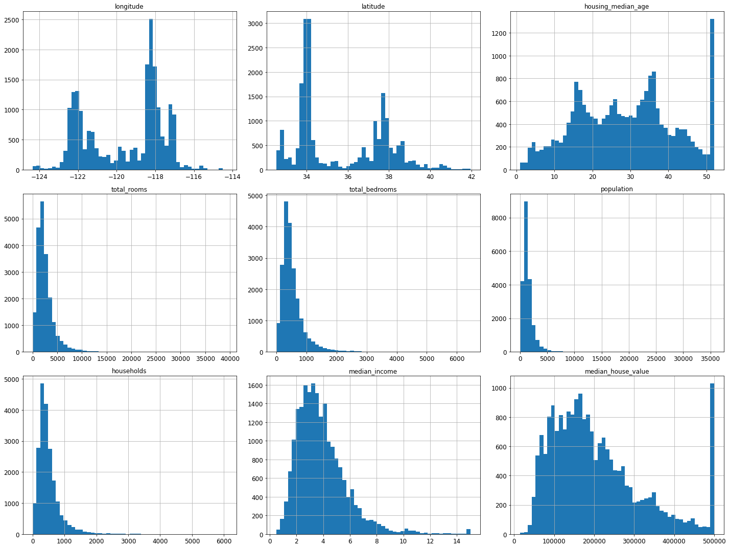
housing.hist(bins=50, figsize=(20,15))
save_fig("attribute_histogram_plots")
plt.show()
Saving figure attribute_histogram_plots
np.random.seed(42)
训练数据:划分
from sklearn.model_selection import train_test_split
train_set, test_set = train_test_split(housing, test_size=0.2, random_state=42)
#test_size=0.2 测试集占20%
####################
#############################################################################
# train_set, test_set = train_test_split(housing, test_size=0.2, random_state=42)
#################################################################################################
train_set.head(5)
| longitude | latitude | housing_median_age | total_rooms | total_bedrooms | population | households | median_income | median_house_value | ocean_proximity | |
|---|---|---|---|---|---|---|---|---|---|---|
| 14196 | -117.03 | 32.71 | 33.0 | 3126.0 | 627.0 | 2300.0 | 623.0 | 3.2596 | 103000.0 | NEAR OCEAN |
| 8267 | -118.16 | 33.77 | 49.0 | 3382.0 | 787.0 | 1314.0 | 756.0 | 3.8125 | 382100.0 | NEAR OCEAN |
| 17445 | -120.48 | 34.66 | 4.0 | 1897.0 | 331.0 | 915.0 | 336.0 | 4.1563 | 172600.0 | NEAR OCEAN |
| 14265 | -117.11 | 32.69 | 36.0 | 1421.0 | 367.0 | 1418.0 | 355.0 | 1.9425 | 93400.0 | NEAR OCEAN |
| 2271 | -119.80 | 36.78 | 43.0 | 2382.0 | 431.0 | 874.0 | 380.0 | 3.5542 | 96500.0 | INLAND |
test_set.head()
| longitude | latitude | housing_median_age | total_rooms | total_bedrooms | population | households | median_income | median_house_value | ocean_proximity | |
|---|---|---|---|---|---|---|---|---|---|---|
| 20046 | -119.01 | 36.06 | 25.0 | 1505.0 | NaN | 1392.0 | 359.0 | 1.6812 | 47700.0 | INLAND |
| 3024 | -119.46 | 35.14 | 30.0 | 2943.0 | NaN | 1565.0 | 584.0 | 2.5313 | 45800.0 | INLAND |
| 15663 | -122.44 | 37.80 | 52.0 | 3830.0 | NaN | 1310.0 | 963.0 | 3.4801 | 500001.0 | NEAR BAY |
| 20484 | -118.72 | 34.28 | 17.0 | 3051.0 | NaN | 1705.0 | 495.0 | 5.7376 | 218600.0 | <1H OCEAN |
| 9814 | -121.93 | 36.62 | 34.0 | 2351.0 | NaN | 1063.0 | 428.0 | 3.7250 | 278000.0 | NEAR OCEAN |
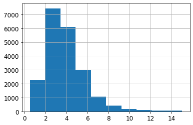
housing["median_income"].hist()
<AxesSubplot:>
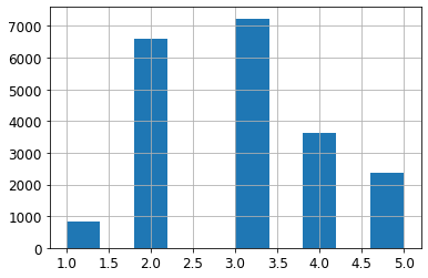
housing['income_cat']= pd.cut(housing['median_income'],bins=[0., 1.5, 3.0, 4.5, 6., np.inf],labels=[1, 2, 3, 4, 5])
housing['income_cat'].value_counts()
3    7236
2    6581
4    3639
5    2362
1     822
Name: income_cat, dtype: int64
housing['income_cat'].hist()
<AxesSubplot:>
https://blog.csdn.net/Cicome/article/details/79153268
使用StratifiedShuffleSplit进行分层采样
from sklearn.model_selection import StratifiedShuffleSplit

split = StratifiedShuffleSplit(n_splits=1, test_size=0.2, random_state=42)
for train_index, test_index in split.split(housing, housing["income_cat"]):
    strat_train_set = housing.loc[train_index]
    strat_test_set = housing.loc[test_index]
###########################################################################
train_index, test_index in split.split(housing, housing["income_cat"])
print(len(train_index),len(test_index))
16512 4128


D:\anaconda\lib\site-packages\ipykernel_launcher.py:2: VisibleDeprecationWarning: Creating an ndarray from ragged nested sequences (which is a list-or-tuple of lists-or-tuples-or ndarrays with different lengths or shapes) is deprecated. If you meant to do this, you must specify 'dtype=object' when creating the ndarray

D:\anaconda\lib\site-packages\ipykernel_launcher.py:2: DeprecationWarning: elementwise comparison failed; this will raise an error in the future.
strat_test_set["income_cat"].value_counts() / len(strat_test_set)
3    0.350533
2    0.318798
4    0.176357
5    0.114583
1    0.039729
Name: income_cat, dtype: float64
for set_ in (strat_train_set, strat_test_set):
    set_.drop("income_cat", axis=1, inplace=True)
数据探索
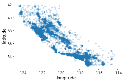
housing = strat_train_set.copy()
housing.plot(kind="scatter", x="longitude", y="latitude",alpha=0.2)
save_fig("bad_visualization_plot")
Saving figure bad_visualization_plot
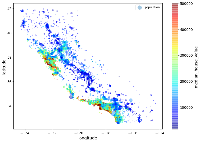
housing.plot(kind="scatter", x="longitude", y="latitude", alpha=0.4,
    s=housing["population"]/100, label="population", figsize=(10,7),
    c="median_house_value", cmap=plt.get_cmap("jet"), colorbar=True,
    sharex=False)
plt.legend()
save_fig("housing_prices_scatterplot")
Saving figure housing_prices_scatterplot
import os
import tarfile
import urllib.request

PROJECT_ROOT_DIR = "."

images_path = os.path.join(PROJECT_ROOT_DIR, "images", "end_to_end_project")
os.makedirs(images_path, exist_ok=True)
DOWNLOAD_ROOT = "https://raw.githubusercontent.com/ageron/handson-ml/master/"
filename = "california.png"
print("Downloading", filename)
url = DOWNLOAD_ROOT + "images/end_to_end_project/" + filename
urllib.request.urlretrieve(url, os.path.join(images_path, filename))
Downloading california.png


('.\\images\\end_to_end_project\\california.png',
 <http.client.HTTPMessage at 0x22a301f6648>)
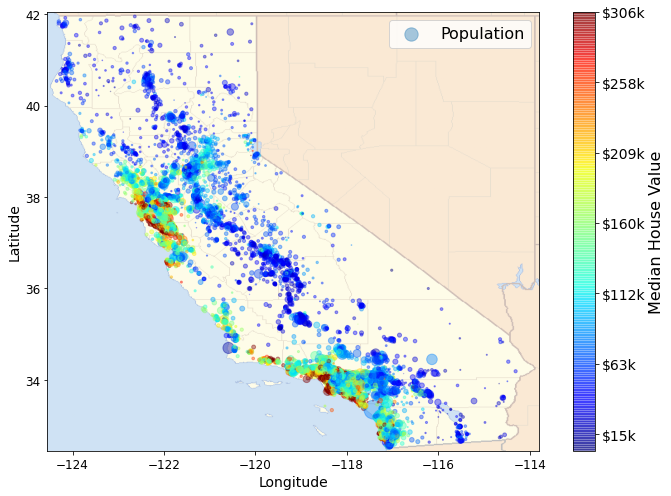
import matplotlib.image as mpimg

california_img=mpimg.imread(PROJECT_ROOT_DIR + '/images/end_to_end_project/california.png')
ax = housing.plot(kind="scatter", x="longitude", y="latitude", figsize=(10,7),
                       s=housing['population']/100, label="Population",
                       c="median_house_value", cmap=plt.get_cmap("jet"),
                       colorbar=False, alpha=0.4,
                      )
plt.imshow(california_img, extent=[-124.55, -113.80, 32.45, 42.05], alpha=0.5,
           cmap=plt.get_cmap("jet"))
plt.ylabel("Latitude", fontsize=14)
plt.xlabel("Longitude", fontsize=14)


prices = housing["median_house_value"]
tick_values = np.linspace(prices.min(), prices.max(), 11)
cbar = plt.colorbar()
cbar.ax.set_yticklabels(["$%dk"%(round(v/1000)) for v in tick_values], fontsize=14)
cbar.set_label('Median House Value', fontsize=16)

plt.legend(fontsize=16)
save_fig("california_housing_prices_plot")
plt.show()
D:\anaconda\lib\site-packages\ipykernel_launcher.py:18: UserWarning: FixedFormatter should only be used together with FixedLocator


Saving figure california_housing_prices_plot
相关系数
corr_matrix = housing.corr()
#每个属性和房价中位数的关联度
corr_matrix["median_house_value"].sort_values(ascending=False)
median_house_value    1.000000
median_income         0.688075
total_rooms           0.134153
housing_median_age    0.105623
households            0.065843
total_bedrooms        0.049686
population           -0.024650
longitude            -0.045967
latitude             -0.144160
Name: median_house_value, dtype: float64
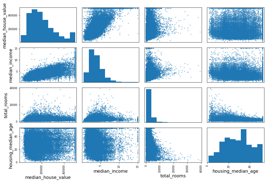
from pandas.plotting import scatter_matrix


attributes = ["median_house_value", "median_income", "total_rooms",
              "housing_median_age"]
scatter_matrix(housing[attributes], figsize=(12, 8))
save_fig("scatter_matrix_plot")
Saving figure scatter_matrix_plot
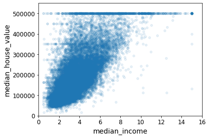
housing.plot(kind="scatter", x="median_income", y="median_house_value",
             alpha=0.1)
plt.axis([0, 16, 0, 550000])
save_fig("income_vs_house_value_scatterplot")
Saving figure income_vs_house_value_scatterplot
属性组合试验
housing["rooms_per_household"] = housing["total_rooms"]/housing["households"]
housing["bedrooms_per_room"] = housing["total_bedrooms"]/housing["total_rooms"]
housing["population_per_household"]=housing["population"]/housing["households"]
corr_matrix = housing.corr()
corr_matrix["median_house_value"].sort_values(ascending=False)
median_house_value          1.000000
median_income               0.688075
rooms_per_household         0.151948
total_rooms                 0.134153
housing_median_age          0.105623
households                  0.065843
total_bedrooms              0.049686
population_per_household   -0.023737
population                 -0.024650
longitude                  -0.045967
latitude                   -0.144160
bedrooms_per_room          -0.255880
Name: median_house_value, dtype: float64
median_house_value
- median_income 0.687160
- bedrooms_per_room -0.259984
- rooms_per_household 0.146285
- total_rooms 0.135097
- housing_median_age 0.114110
Prepare the data for Machine Learning algorithms
- 在任何数据集上(比如,你下一次获取的是一个新的数据集)方便地进行重复数据转换。
- 慢慢建立一个转换函数库,可以在未来的项目中复用。
housing = strat_train_set.drop("median_house_value", axis=1) # 不影响原数据,只会建立备份
housing_labels = strat_train_set["median_house_value"].copy()
数据清洗
对于缺失值:
- 去掉对应的街区;
- 去掉整个属性;
- 进行赋值(0、平均值、中位数等等)。
housing.dropna(subset=["total_bedrooms"]) # 选项1
housing.drop("total_bedrooms", axis=1) # 选项2
median = housing["total_bedrooms"].median()
housing["total_bedrooms"].fillna(median) # 选项3
如果选择选项 3,你需要计算训练集的中位数,用中位数填充训练集的缺失值,不要忘记保存
该中位数。后面用测试集评估系统时,需要替换测试集中的缺失值,也可以用来实时替换新
数据中的缺失值
Scikit-Learn 提供了一个方便的类来处理缺失值: Imputer
from sklearn.preprocessing import Imputer
imputer = Imputer(strategy="median")
housing_num = housing.drop("ocean_proximity", axis=1)
imputer.fit(housing_num)
imputer.statistics_
X = imputer.transform(housing_num)
housing_tr = pd.DataFrame(X, columns=housing_num.columns)
sample_incomplete_rows = housing[housing.isnull().any(axis=1)].head()
#df.isnull().any()会判断哪些列包含缺失值
sample_incomplete_rows
| longitude | latitude | housing_median_age | total_rooms | total_bedrooms | population | households | median_income | ocean_proximity | |
|---|---|---|---|---|---|---|---|---|---|
| 4629 | -118.30 | 34.07 | 18.0 | 3759.0 | NaN | 3296.0 | 1462.0 | 2.2708 | <1H OCEAN |
| 6068 | -117.86 | 34.01 | 16.0 | 4632.0 | NaN | 3038.0 | 727.0 | 5.1762 | <1H OCEAN |
| 17923 | -121.97 | 37.35 | 30.0 | 1955.0 | NaN | 999.0 | 386.0 | 4.6328 | <1H OCEAN |
| 13656 | -117.30 | 34.05 | 6.0 | 2155.0 | NaN | 1039.0 | 391.0 | 1.6675 | INLAND |
| 19252 | -122.79 | 38.48 | 7.0 | 6837.0 | NaN | 3468.0 | 1405.0 | 3.1662 | <1H OCEAN |
可见total_bedrooms存在缺失值
于是用中位数代替
正好把数据集里所有的特征的中位数一起算了
保存在Imputer里
这里用异常处理一下sklearn版本更迭的问题
try:
    from sklearn.impute import SimpleImputer # Scikit-Learn 0.20+
except ImportError:
    from sklearn.preprocessing import Imputer as SimpleImputer

imputer = SimpleImputer(strategy="median")
housing_num = housing.drop('ocean_proximity', axis=1)#把标量数据删除,不然没法统一算中位数
imputer.fit(housing_num)
SimpleImputer(strategy='median')
#看看数据
imputer.statistics_
array([-118.51  ,   34.26  ,   29.    , 2119.5   ,  433.    , 1164.    ,
        408.    ,    3.5409])
X = imputer.transform(housing_num)#将缺失值替换为中位数
housing_num
| longitude | latitude | housing_median_age | total_rooms | total_bedrooms | population | households | median_income | |
|---|---|---|---|---|---|---|---|---|
| 17606 | -121.89 | 37.29 | 38.0 | 1568.0 | 351.0 | 710.0 | 339.0 | 2.7042 |
| 18632 | -121.93 | 37.05 | 14.0 | 679.0 | 108.0 | 306.0 | 113.0 | 6.4214 |
| 14650 | -117.20 | 32.77 | 31.0 | 1952.0 | 471.0 | 936.0 | 462.0 | 2.8621 |
| 3230 | -119.61 | 36.31 | 25.0 | 1847.0 | 371.0 | 1460.0 | 353.0 | 1.8839 |
| 3555 | -118.59 | 34.23 | 17.0 | 6592.0 | 1525.0 | 4459.0 | 1463.0 | 3.0347 |
| ... | ... | ... | ... | ... | ... | ... | ... | ... |
| 6563 | -118.13 | 34.20 | 46.0 | 1271.0 | 236.0 | 573.0 | 210.0 | 4.9312 |
| 12053 | -117.56 | 33.88 | 40.0 | 1196.0 | 294.0 | 1052.0 | 258.0 | 2.0682 |
| 13908 | -116.40 | 34.09 | 9.0 | 4855.0 | 872.0 | 2098.0 | 765.0 | 3.2723 |
| 11159 | -118.01 | 33.82 | 31.0 | 1960.0 | 380.0 | 1356.0 | 356.0 | 4.0625 |
| 15775 | -122.45 | 37.77 | 52.0 | 3095.0 | 682.0 | 1269.0 | 639.0 | 3.5750 |
16512 rows × 8 columns
housing_tr = pd.DataFrame(X, columns=housing_num.columns,
                          index=housing.index)
处理标量数据
housing_cat = housing[['ocean_proximity']]
housing_cat.head(10)
| ocean_proximity | |
|---|---|
| 17606 | <1H OCEAN |
| 18632 | <1H OCEAN |
| 14650 | NEAR OCEAN |
| 3230 | INLAND |
| 3555 | <1H OCEAN |
| 19480 | INLAND |
| 8879 | <1H OCEAN |
| 13685 | INLAND |
| 4937 | <1H OCEAN |
| 4861 | <1H OCEAN |
try:
    from sklearn.preprocessing import OrdinalEncoder # just to raise an ImportError if Scikit-Learn < 0.20
    from sklearn.preprocessing import OneHotEncoder
except ImportError:
    from future_encoders import OneHotEncoder

cat_encoder = OneHotEncoder(sparse=False)
housing_cat_1hot = cat_encoder.fit_transform(housing_cat)
housing_cat_1hot
array([[1., 0., 0., 0., 0.],
       [1., 0., 0., 0., 0.],
       [0., 0., 0., 0., 1.],
       ...,
       [0., 1., 0., 0., 0.],
       [1., 0., 0., 0., 0.],
       [0., 0., 0., 1., 0.]])
housing.columns
Index(['longitude', 'latitude', 'housing_median_age', 'total_rooms',
       'total_bedrooms', 'population', 'households', 'median_income',
       'ocean_proximity'],
      dtype='object')
创建自己的类
自定义转换函器:
创建一个类,实现fit()[return self]、transform()和fit_transform()
通过添加 TransformerMixin 作为基类(父类),可以很容易地得到fit_transform()。
另外,如果你添加 BaseEstimator 作为基类(父类)(且构造器中避免使用 *args 和 **kargs ),你就能得到两个额外的方法( get_params() 和 set_params() ),
二者可以方便地进行超参数自动微调
sklearn项目可以看成一棵大树,各种estimator是果实,而支撑这些估计器的主干,是为数不多的几个基类。常见的几个类有BaseEstimator、BaseSGD、ClassifierMixin、RegressorMixin,等等。[origin]https://www.cnblogs.com/learn-the-hard-way/p/12532888.html
np.c_ 把几个array连在一起
from sklearn.base import BaseEstimator, TransformerMixin

# get the right column indices: safer than hard-coding indices 3, 4, 5, 6
rooms_ix, bedrooms_ix, population_ix, household_ix = [
    list(housing.columns).index(col)
    for col in ("total_rooms", "total_bedrooms", "population", "households")]

class CombinedAttributesAdder(BaseEstimator, TransformerMixin):
    def __init__(self, add_bedrooms_per_room = True): # no *args or **kwargs
        self.add_bedrooms_per_room = add_bedrooms_per_room
    def fit(self, X, y=None):
        return self  # nothing else to do
    def transform(self, X, y=None):
        rooms_per_household = X[:, rooms_ix] / X[:, household_ix]
        population_per_household = X[:, population_ix] / X[:, household_ix]
        if self.add_bedrooms_per_room:
            bedrooms_per_room = X[:, bedrooms_ix] / X[:, rooms_ix]
            return np.c_[X, rooms_per_household, population_per_household,
                         bedrooms_per_room]
        #  np.c_ 把几个array连在一起
        else:
            return np.c_[X, rooms_per_household, population_per_household]

attr_adder = CombinedAttributesAdder(add_bedrooms_per_room=False)
housing_extra_attribs = attr_adder.transform(housing.values)
另一种方法:FunctionTransformer
from sklearn.preprocessing import FunctionTransformer

def add_extra_features(X, add_bedrooms_per_room=True):
    rooms_per_household = X[:, rooms_ix] / X[:, household_ix]
    population_per_household = X[:, population_ix] / X[:, household_ix]
    if add_bedrooms_per_room:
        bedrooms_per_room = X[:, bedrooms_ix] / X[:, rooms_ix]
        return np.c_[X, rooms_per_household, population_per_household,
                     bedrooms_per_room]
    else:
        return np.c_[X, rooms_per_household, population_per_household]

attr_adder = FunctionTransformer(add_extra_features, validate=False,
                                 kw_args={"add_bedrooms_per_room": False})
housing_extra_attribs = attr_adder.fit_transform(housing.values)
housing_extra_attribs = pd.DataFrame(
    housing_extra_attribs,
    columns=list(housing.columns)+["rooms_per_household", "population_per_household"],
    index=housing.index)
housing_extra_attribs.columns
Index(['longitude', 'latitude', 'housing_median_age', 'total_rooms',
       'total_bedrooms', 'population', 'households', 'median_income',
       'ocean_proximity', 'rooms_per_household', 'population_per_household'],
      dtype='object')
from sklearn.pipeline import Pipeline
from sklearn.preprocessing import StandardScaler

num_pipeline = Pipeline([
        ('imputer', SimpleImputer(strategy="median")),#1.去除缺失值  #执行     imputer = SimpleImputer(strategy="median")   imputer.fit(housing_num)
        ('attribs_adder', FunctionTransformer(add_extra_features, validate=False)),#2.添加属性     #FunctionTransformer(add_extra_features, validate=False)
        ('std_scaler', StandardScaler()),#3.特征缩放
    ])

housing_num_tr = num_pipeline.fit_transform(housing_num)
Index(['longitude', 'latitude', 'housing_median_age', 'total_rooms',
       'total_bedrooms', 'population', 'households', 'median_income'],
      dtype='object')
特征缩放
机器学习中重要的一个环节
暂时不进行更新
转换流水线
使用pipline按一定的顺序执行程序
try:
    from sklearn.compose import ColumnTransformer
except ImportError:
    from future_encoders import ColumnTransformer # Scikit-Learn < 0.20
num_attribs = list(housing_num)
cat_attribs = ["ocean_proximity"]

full_pipeline = ColumnTransformer([
        ("num", num_pipeline, num_attribs),
        ("cat", OneHotEncoder(), cat_attribs),
    ])

housing_prepared = full_pipeline.fit_transform(housing)
housing_prepared
array([[-1.15604281,  0.77194962,  0.74333089, ...,  0.        ,
         0.        ,  0.        ],
       [-1.17602483,  0.6596948 , -1.1653172 , ...,  0.        ,
         0.        ,  0.        ],
       [ 1.18684903, -1.34218285,  0.18664186, ...,  0.        ,
         0.        ,  1.        ],
       ...,
       [ 1.58648943, -0.72478134, -1.56295222, ...,  0.        ,
         0.        ,  0.        ],
       [ 0.78221312, -0.85106801,  0.18664186, ...,  0.        ,
         0.        ,  0.        ],
       [-1.43579109,  0.99645926,  1.85670895, ...,  0.        ,
         1.        ,  0.        ]])
housing_prepared.shape
(16512, 16)
from sklearn.base import BaseEstimator, TransformerMixin

# Create a class to select numerical or categorical columns
class OldDataFrameSelector(BaseEstimator, TransformerMixin):
    def __init__(self, attribute_names):
        self.attribute_names = attribute_names
    def fit(self, X, y=None):
        return self
    def transform(self, X):
        return X[self.attribute_names].values
num_attribs = list(housing_num)
cat_attribs = ["ocean_proximity"]

old_num_pipeline = Pipeline([
        ('selector', OldDataFrameSelector(num_attribs)),
        ('imputer', SimpleImputer(strategy="median")),
        ('attribs_adder', FunctionTransformer(add_extra_features, validate=False)),
        ('std_scaler', StandardScaler()),
    ])

old_cat_pipeline = Pipeline([
        ('selector', OldDataFrameSelector(cat_attribs)),
        ('cat_encoder', OneHotEncoder(sparse=False)),
    ])
from sklearn.pipeline import FeatureUnion

old_full_pipeline = FeatureUnion(transformer_list=[
        ("num_pipeline", old_num_pipeline),
        ("cat_pipeline", old_cat_pipeline),
    ])
old_housing_prepared = old_full_pipeline.fit_transform(housing)
old_housing_prepared
array([[-1.15604281,  0.77194962,  0.74333089, ...,  0.        ,
         0.        ,  0.        ],
       [-1.17602483,  0.6596948 , -1.1653172 , ...,  0.        ,
         0.        ,  0.        ],
       [ 1.18684903, -1.34218285,  0.18664186, ...,  0.        ,
         0.        ,  1.        ],
       ...,
       [ 1.58648943, -0.72478134, -1.56295222, ...,  0.        ,
         0.        ,  0.        ],
       [ 0.78221312, -0.85106801,  0.18664186, ...,  0.        ,
         0.        ,  0.        ],
       [-1.43579109,  0.99645926,  1.85670895, ...,  0.        ,
         1.        ,  0.        ]])
np.allclose(housing_prepared, old_housing_prepared)
True
选择并训练模型
from sklearn.linear_model import LinearRegression

lin_reg = LinearRegression()
lin_reg.fit(housing_prepared, housing_labels)
LinearRegression()
some_data=housing.iloc[:5]
some_labels=housing_labels.iloc[:5]
some_data_prepared = full_pipeline.transform(some_data)

print("Predictions:", lin_reg.predict(some_data_prepared))
Predictions: [210644.60459286 317768.80697211 210956.43331178  59218.98886849
 189747.55849879]
from sklearn.metrics import mean_squared_error

housing_predictions = lin_reg.predict(housing_prepared)
lin_mse = mean_squared_error(housing_labels, housing_predictions)
lin_rmse = np.sqrt(lin_mse)
lin_rmse
68628.19819848923
68628.19819848923
median housing value 位于120000 与 265000 之间
因此68628还是太大了!!!!
意味着这个模型出现了欠拟合的问题
修复欠拟合的主要方法是选择一个更强大的模型,给训练算法提供更好的特征,或去掉模型上的限制。这个模型还没有正则化,所以排除了最后一个选项。你可以尝试添加更多特征(比如,人口的对数值),但是首先让我们尝试一个更为复杂的模型,看看效果。
试试决策树
from sklearn.tree import DecisionTreeRegressor

tree_reg = DecisionTreeRegressor(random_state=42)
tree_reg.fit(housing_prepared, housing_labels)
DecisionTreeRegressor(random_state=42)
housing_predictions = tree_reg.predict(housing_prepared)
tree_mse = mean_squared_error(housing_labels, housing_predictions)
tree_rmse = np.sqrt(tree_mse)
tree_rmse
0.0
RMSE竟然是0!!!!!!!!!!!!!!!!!!!
严重过拟合预警!!!!!!!!!!!!!
在我们选定好模型之前,不能碰测试集一丝一毫!!!!!!!
交叉验证
from sklearn.model_selection import cross_val_score

scores = cross_val_score(tree_reg, housing_prepared, housing_labels,
                         scoring="neg_mean_squared_error", cv=10)
tree_rmse_scores = np.sqrt(-scores)
特别批注!!!!!!!!!!!!!!
交叉验证得分使用的函数是效用函数,不是代价函数,因此得分越大越好(负数)
计算平方根之前先计算 -scores 。
def display_scores(scores):
    print("Scores:", scores)
    print("Mean:", scores.mean())
    print("Standard deviation:", scores.std())

display_scores(tree_rmse_scores)
Scores: [70194.33680785 66855.16363941 72432.58244769 70758.73896782
 71115.88230639 75585.14172901 70262.86139133 70273.6325285
 75366.87952553 71231.65726027]
Mean: 71407.68766037929
Standard deviation: 2439.4345041191004
看起来比线性回归模型还糟!注意到交叉验证不仅可以让你得到模型性能的评估,还能测量评估的准确性(即,它的标准差)。
决策树的评分大约是 71407,通常波动有 ±2439。
lin_scores = cross_val_score(lin_reg, housing_prepared, housing_labels,
                         scoring="neg_mean_squared_error", cv=10)
lin_rmse_scores = np.sqrt(-lin_scores)
display_scores(lin_rmse_scores)
Scores: [66782.73843989 66960.118071   70347.95244419 74739.57052552
 68031.13388938 71193.84183426 64969.63056405 68281.61137997
 71552.91566558 67665.10082067]
Mean: 69052.46136345083
Standard deviation: 2731.674001798349
线性回归的评分大约是 69052,通常波动有 ±2731。
决策树模型过拟合很严重,它的性能比线性回归模型还差。
from sklearn.ensemble import RandomForestRegressor

forest_reg = RandomForestRegressor(n_estimators=10, random_state=42)
forest_reg.fit(housing_prepared, housing_labels)
RandomForestRegressor(n_estimators=10, random_state=42)
housing_predictions = forest_reg.predict(housing_prepared)
forest_mse = mean_squared_error(housing_labels, housing_predictions)
forest_rmse = np.sqrt(forest_mse)
forest_rmse
21933.31414779769
from sklearn.model_selection import cross_val_score

forest_scores = cross_val_score(forest_reg, housing_prepared, housing_labels,
                                scoring="neg_mean_squared_error", cv=10)
forest_rmse_scores = np.sqrt(-forest_scores)
display_scores(forest_rmse_scores)
Scores: [51646.44545909 48940.60114882 53050.86323649 54408.98730149
 50922.14870785 56482.50703987 51864.52025526 49760.85037653
 55434.21627933 53326.10093303]
Mean: 52583.72407377466
Standard deviation: 2298.353351147122
随机森林的评分大约是 52583,通常波动有 ±2298。
我们这里所说的评分指的是验证集的分数
训练集的评分比验证集的评分低,说明过拟合
解决过拟合可以通过简化模型,给模型加限制(即,规整化),或用更多的训练数据。
在深入随机森林之前,你应该尝试下机器学习算法的其它类型模型(不同核心的支持向量机,神经网络,等等),
不要在调节超参数上花费太多时间。目标是列出一个可能模型的列表(两到五个)。
替换模型比调参优先
你要保存每个试验过的模型,以便后续可以再用。要确保有超参数和训练参数,
以及交叉验证评分,和实际的预测值。这可以让你比较不同类型模型的评分,还可以比
较误差种类。你可以用 Python 的模块pickle,非常方便地保存 Scikit-Learn 模型,或使用sklearn.externals.joblib,后者序列化大 NumPy 数组更有效率:
from sklearn.externals import joblib
joblib.dump(my_model, "my_model.pkl")
# 然后
my_model_loaded = joblib.load("my_model.pkl")
模型微调
假设你现在有了一个列表,列表里有几个有希望的模型。你现在需要对它们进行微调。让我们来看几种微调的方法。
网格搜索
微调的一种方法是手工调整超参数,直到找到一个好的超参数组合。这么做的话会非常冗
长,你也可能没有时间探索多种组合。
你应该使用 Scikit-Learn 的 GridSearchCV 来做这项搜索工作。你所需要做的是告诉 GridSearchCV 要试验有哪些超参数,要试验什么值, GridSearchCV 就能用交叉验证试验所有可能超参数值的组合。例如,下面的代码搜索了 RandomForestRegressor 超参数值的最佳组合:
from sklearn.model_selection import GridSearchCV

param_grid = [
    # try 12 (3×4) combinations of hyperparameters
    {'n_estimators': [3, 10, 30], 'max_features': [2, 4, 6, 8]},
    # then try 6 (2×3) combinations with bootstrap set as False
    {'bootstrap': [False], 'n_estimators': [3, 10], 'max_features': [2, 3, 4]},
  ]

forest_reg = RandomForestRegressor(random_state=42)
# train across 5 folds, that's a total of (12+6)*5=90 rounds of training
grid_search = GridSearchCV(forest_reg, param_grid, cv=5,
                           scoring='neg_mean_squared_error', return_train_score=True)
grid_search.fit(housing_prepared, housing_labels)
GridSearchCV(cv=5, estimator=RandomForestRegressor(random_state=42),
             param_grid=[{'max_features': [2, 4, 6, 8],
                          'n_estimators': [3, 10, 30]},
                         {'bootstrap': [False], 'max_features': [2, 3, 4],
                          'n_estimators': [3, 10]}],
             return_train_score=True, scoring='neg_mean_squared_error')
grid_search.best_params_
{'max_features': 8, 'n_estimators': 30}
grid_search.best_estimator_
RandomForestRegressor(max_features=8, n_estimators=30, random_state=42)
cvres = grid_search.cv_results_
for mean_score, params in zip(cvres["mean_test_score"], cvres["params"]):
    print(np.sqrt(-mean_score), params)
63669.11631261028 {'max_features': 2, 'n_estimators': 3}
55627.099719926795 {'max_features': 2, 'n_estimators': 10}
53384.57275149205 {'max_features': 2, 'n_estimators': 30}
60965.950449450494 {'max_features': 4, 'n_estimators': 3}
52741.04704299915 {'max_features': 4, 'n_estimators': 10}
50377.40461678399 {'max_features': 4, 'n_estimators': 30}
58663.93866579625 {'max_features': 6, 'n_estimators': 3}
52006.19873526564 {'max_features': 6, 'n_estimators': 10}
50146.51167415009 {'max_features': 6, 'n_estimators': 30}
57869.25276169646 {'max_features': 8, 'n_estimators': 3}
51711.127883959234 {'max_features': 8, 'n_estimators': 10}
49682.273345071546 {'max_features': 8, 'n_estimators': 30}
62895.06951262424 {'bootstrap': False, 'max_features': 2, 'n_estimators': 3}
54658.176157539405 {'bootstrap': False, 'max_features': 2, 'n_estimators': 10}
59470.40652318466 {'bootstrap': False, 'max_features': 3, 'n_estimators': 3}
52724.9822587892 {'bootstrap': False, 'max_features': 3, 'n_estimators': 10}
57490.5691951261 {'bootstrap': False, 'max_features': 4, 'n_estimators': 3}
51009.495668875716 {'bootstrap': False, 'max_features': 4, 'n_estimators': 10}
pd.DataFrame(grid_search.cv_results_)
| mean_fit_time | std_fit_time | mean_score_time | std_score_time | param_max_features | param_n_estimators | param_bootstrap | params | split0_test_score | split1_test_score | ... | mean_test_score | std_test_score | rank_test_score | split0_train_score | split1_train_score | split2_train_score | split3_train_score | split4_train_score | mean_train_score | std_train_score | |
|---|---|---|---|---|---|---|---|---|---|---|---|---|---|---|---|---|---|---|---|---|---|
| 0 | 0.066756 | 0.003714 | 0.003599 | 0.000495 | 2 | 3 | NaN | {'max_features': 2, 'n_estimators': 3} | -3.837622e+09 | -4.147108e+09 | ... | -4.053756e+09 | 1.519591e+08 | 18 | -1.064113e+09 | -1.105142e+09 | -1.116550e+09 | -1.112342e+09 | -1.129650e+09 | -1.105559e+09 | 2.220402e+07 |
| 1 | 0.214235 | 0.007558 | 0.010251 | 0.001075 | 2 | 10 | NaN | {'max_features': 2, 'n_estimators': 10} | -3.047771e+09 | -3.254861e+09 | ... | -3.094374e+09 | 1.327062e+08 | 11 | -5.927175e+08 | -5.870952e+08 | -5.776964e+08 | -5.716332e+08 | -5.802501e+08 | -5.818785e+08 | 7.345821e+06 |
| 2 | 0.670176 | 0.023281 | 0.027710 | 0.001455 | 2 | 30 | NaN | {'max_features': 2, 'n_estimators': 30} | -2.689185e+09 | -3.021086e+09 | ... | -2.849913e+09 | 1.626875e+08 | 9 | -4.381089e+08 | -4.391272e+08 | -4.371702e+08 | -4.376955e+08 | -4.452654e+08 | -4.394734e+08 | 2.966320e+06 |
| 3 | 0.117089 | 0.017003 | 0.003790 | 0.000399 | 4 | 3 | NaN | {'max_features': 4, 'n_estimators': 3} | -3.730181e+09 | -3.786886e+09 | ... | -3.716847e+09 | 1.631510e+08 | 16 | -9.865163e+08 | -1.012565e+09 | -9.169425e+08 | -1.037400e+09 | -9.707739e+08 | -9.848396e+08 | 4.084607e+07 |
| 4 | 0.366152 | 0.056251 | 0.009570 | 0.000797 | 4 | 10 | NaN | {'max_features': 4, 'n_estimators': 10} | -2.666283e+09 | -2.784511e+09 | ... | -2.781618e+09 | 1.268607e+08 | 8 | -5.097115e+08 | -5.162820e+08 | -4.962893e+08 | -5.436192e+08 | -5.160297e+08 | -5.163863e+08 | 1.542862e+07 |
| 5 | 0.997333 | 0.014813 | 0.027328 | 0.000798 | 4 | 30 | NaN | {'max_features': 4, 'n_estimators': 30} | -2.387153e+09 | -2.588448e+09 | ... | -2.537883e+09 | 1.214614e+08 | 3 | -3.838835e+08 | -3.880268e+08 | -3.790867e+08 | -4.040957e+08 | -3.845520e+08 | -3.879289e+08 | 8.571233e+06 |
| 6 | 0.138494 | 0.007538 | 0.003989 | 0.001093 | 6 | 3 | NaN | {'max_features': 6, 'n_estimators': 3} | -3.119657e+09 | -3.586319e+09 | ... | -3.441458e+09 | 1.893056e+08 | 14 | -9.245343e+08 | -8.886939e+08 | -9.353135e+08 | -9.009801e+08 | -8.624664e+08 | -9.023976e+08 | 2.591445e+07 |
| 7 | 0.481576 | 0.026511 | 0.010872 | 0.002037 | 6 | 10 | NaN | {'max_features': 6, 'n_estimators': 10} | -2.549663e+09 | -2.782039e+09 | ... | -2.704645e+09 | 1.471569e+08 | 6 | -4.980344e+08 | -5.045869e+08 | -4.994664e+08 | -4.990325e+08 | -5.055542e+08 | -5.013349e+08 | 3.100456e+06 |
| 8 | 1.588877 | 0.041150 | 0.035582 | 0.007298 | 6 | 30 | NaN | {'max_features': 6, 'n_estimators': 30} | -2.370010e+09 | -2.583638e+09 | ... | -2.514673e+09 | 1.285080e+08 | 2 | -3.838538e+08 | -3.804711e+08 | -3.805218e+08 | -3.856095e+08 | -3.901917e+08 | -3.841296e+08 | 3.617057e+06 |
| 9 | 0.206154 | 0.005440 | 0.004792 | 0.000748 | 8 | 3 | NaN | {'max_features': 8, 'n_estimators': 3} | -3.353504e+09 | -3.348552e+09 | ... | -3.348850e+09 | 1.241939e+08 | 13 | -9.228123e+08 | -8.553031e+08 | -8.603321e+08 | -8.881964e+08 | -9.151287e+08 | -8.883545e+08 | 2.750227e+07 |
| 10 | 0.730898 | 0.079985 | 0.013963 | 0.001784 | 8 | 10 | NaN | {'max_features': 8, 'n_estimators': 10} | -2.571970e+09 | -2.718994e+09 | ... | -2.674041e+09 | 1.392777e+08 | 5 | -4.932416e+08 | -4.815238e+08 | -4.730979e+08 | -5.155367e+08 | -4.985555e+08 | -4.923911e+08 | 1.459294e+07 |
| 11 | 1.927305 | 0.084095 | 0.031714 | 0.001329 | 8 | 30 | NaN | {'max_features': 8, 'n_estimators': 30} | -2.357390e+09 | -2.546640e+09 | ... | -2.468328e+09 | 1.091662e+08 | 1 | -3.841658e+08 | -3.744500e+08 | -3.773239e+08 | -3.882250e+08 | -3.810005e+08 | -3.810330e+08 | 4.871017e+06 |
| 12 | 0.112344 | 0.002530 | 0.004182 | 0.000400 | 2 | 3 | False | {'bootstrap': False, 'max_features': 2, 'n_est... | -3.785816e+09 | -4.166012e+09 | ... | -3.955790e+09 | 1.900964e+08 | 17 | -0.000000e+00 | -0.000000e+00 | -0.000000e+00 | -0.000000e+00 | -0.000000e+00 | 0.000000e+00 | 0.000000e+00 |
| 13 | 0.373254 | 0.006915 | 0.011758 | 0.000744 | 2 | 10 | False | {'bootstrap': False, 'max_features': 2, 'n_est... | -2.810721e+09 | -3.107789e+09 | ... | -2.987516e+09 | 1.539234e+08 | 10 | -6.056477e-02 | -0.000000e+00 | -0.000000e+00 | -0.000000e+00 | -2.967449e+00 | -6.056027e-01 | 1.181156e+00 |
| 14 | 0.146921 | 0.007771 | 0.004595 | 0.000791 | 3 | 3 | False | {'bootstrap': False, 'max_features': 3, 'n_est... | -3.618324e+09 | -3.441527e+09 | ... | -3.536729e+09 | 7.795057e+07 | 15 | -0.000000e+00 | -0.000000e+00 | -0.000000e+00 | -0.000000e+00 | -6.072840e+01 | -1.214568e+01 | 2.429136e+01 |
| 15 | 0.456709 | 0.005146 | 0.011781 | 0.000736 | 3 | 10 | False | {'bootstrap': False, 'max_features': 3, 'n_est... | -2.757999e+09 | -2.851737e+09 | ... | -2.779924e+09 | 6.286720e+07 | 7 | -2.089484e+01 | -0.000000e+00 | -0.000000e+00 | -0.000000e+00 | -5.465556e+00 | -5.272080e+00 | 8.093117e+00 |
| 16 | 0.172073 | 0.001793 | 0.004594 | 0.000792 | 4 | 3 | False | {'bootstrap': False, 'max_features': 4, 'n_est... | -3.134040e+09 | -3.559375e+09 | ... | -3.305166e+09 | 1.879165e+08 | 12 | -0.000000e+00 | -0.000000e+00 | -0.000000e+00 | -0.000000e+00 | -0.000000e+00 | 0.000000e+00 | 0.000000e+00 |
| 17 | 0.564507 | 0.008674 | 0.012361 | 0.000795 | 4 | 10 | False | {'bootstrap': False, 'max_features': 4, 'n_est... | -2.525578e+09 | -2.710011e+09 | ... | -2.601969e+09 | 1.088048e+08 | 4 | -0.000000e+00 | -1.514119e-02 | -0.000000e+00 | -0.000000e+00 | -0.000000e+00 | -3.028238e-03 | 6.056477e-03 |
18 rows × 23 columns
成功地微调了最佳模型
提示:不要忘记,你可以像超参数一样处理数据准备的步骤。例如,网格搜索可以自动
判断是否添加一个你不确定的特征(比如,使用转换器 CombinedAttributesAdder 的超参
数 add_bedrooms_per_room )。它还能用相似的方法来自动找到处理异常值、缺失特征、
特征选择等任务的最佳方法。
随机搜索
超参数的搜索空间很大时,最好使用 RandomizedSearchCV
from sklearn.model_selection import RandomizedSearchCV
from scipy.stats import randint

param_distribs = {
        'n_estimators': randint(low=1, high=200),
        'max_features': randint(low=1, high=8),
    }

forest_reg = RandomForestRegressor(random_state=42)
rnd_search = RandomizedSearchCV(forest_reg, param_distributions=param_distribs,
                                n_iter=10, cv=5, scoring='neg_mean_squared_error', random_state=42)
rnd_search.fit(housing_prepared, housing_labels)
RandomizedSearchCV(cv=5, estimator=RandomForestRegressor(random_state=42),
                   param_distributions={'max_features': <scipy.stats._distn_infrastructure.rv_frozen object at 0x000001FAB8188D88>,
                                        'n_estimators': <scipy.stats._distn_infrastructure.rv_frozen object at 0x000001FAB8188C08>},
                   random_state=42, scoring='neg_mean_squared_error')
cvres = rnd_search.cv_results_
for mean_score, params in zip(cvres["mean_test_score"], cvres["params"]):
    print(np.sqrt(-mean_score), params)
49150.70756927707 {'max_features': 7, 'n_estimators': 180}
51389.889203389284 {'max_features': 5, 'n_estimators': 15}
50796.155224308866 {'max_features': 3, 'n_estimators': 72}
50835.13360315349 {'max_features': 5, 'n_estimators': 21}
49280.9449827171 {'max_features': 7, 'n_estimators': 122}
50774.90662363929 {'max_features': 3, 'n_estimators': 75}
50682.78888164288 {'max_features': 3, 'n_estimators': 88}
49608.99608105296 {'max_features': 5, 'n_estimators': 100}
50473.61930350219 {'max_features': 3, 'n_estimators': 150}
64429.84143294435 {'max_features': 5, 'n_estimators': 2}
每个属性(特征)对于做出准确预测的相对重要性
feature_importances = grid_search.best_estimator_.feature_importances_
feature_importances
array([7.33442355e-02, 6.29090705e-02, 4.11437985e-02, 1.46726854e-02,
       1.41064835e-02, 1.48742809e-02, 1.42575993e-02, 3.66158981e-01,
       5.64191792e-02, 1.08792957e-01, 5.33510773e-02, 1.03114883e-02,
       1.64780994e-01, 6.02803867e-05, 1.96041560e-03, 2.85647464e-03])
extra_attribs = ["rooms_per_hhold", "pop_per_hhold", "bedrooms_per_room"]
#cat_encoder = cat_pipeline.named_steps["cat_encoder"] # old solution
cat_encoder = full_pipeline.named_transformers_["cat"]
cat_one_hot_attribs = list(cat_encoder.categories_[0])
attributes = num_attribs + extra_attribs + cat_one_hot_attribs
sorted(zip(feature_importances, attributes), reverse=True)
[(0.36615898061813423, 'median_income'),
 (0.16478099356159054, 'INLAND'),
 (0.10879295677551575, 'pop_per_hhold'),
 (0.07334423551601243, 'longitude'),
 (0.06290907048262032, 'latitude'),
 (0.056419179181954014, 'rooms_per_hhold'),
 (0.053351077347675815, 'bedrooms_per_room'),
 (0.04114379847872964, 'housing_median_age'),
 (0.014874280890402769, 'population'),
 (0.014672685420543239, 'total_rooms'),
 (0.014257599323407808, 'households'),
 (0.014106483453584104, 'total_bedrooms'),
 (0.010311488326303788, '<1H OCEAN'),
 (0.0028564746373201584, 'NEAR OCEAN'),
 (0.0019604155994780706, 'NEAR BAY'),
 (6.0280386727366e-05, 'ISLAND')]
final_model = grid_search.best_estimator_

X_test = strat_test_set.drop("median_house_value", axis=1)
y_test = strat_test_set["median_house_value"].copy()

X_test_prepared = full_pipeline.transform(X_test)
final_predictions = final_model.predict(X_test_prepared)

final_mse = mean_squared_error(y_test, final_predictions)
final_rmse = np.sqrt(final_mse)
计算RMSE的置信区间
from scipy import stats

confidence = 0.95
squared_errors = (final_predictions - y_test) ** 2
mean = squared_errors.mean()
m = len(squared_errors)

np.sqrt(stats.t.interval(confidence, m - 1,
                         loc=np.mean(squared_errors),
                         scale=stats.sem(squared_errors)))
array([45685.10470776, 49691.25001878])


 876
876


 被折叠的 条评论
为什么被折叠?
被折叠的 条评论
为什么被折叠?
 到【灌水乐园】发言


