机器学习回归与聚类算法

最新推荐文章于 2023-06-13 10:00:04 发布

可爱的杨一凡

最新推荐文章于 2023-06-13 10:00:04 发布

阅读量228

点赞数 1

分类专栏：人工智能文章标签：机器学习回归算法

本文链接：https://blog.csdn.net/weixin_45553177/article/details/122164593

版权

人工智能专栏收录该内容

3 篇文章 0 订阅

订阅专栏

机器学习回归与聚类算法

思维导图

线性回归
欠拟合与过拟合
岭回归

分类算法：逻辑回归

模型保存与加载

无监督学习 K-means算法

4.1 线性回归

回归问题：
    目标值 - 连续型的数据

4.1.1 线性回归的原理

    2 什么是线性回归
        函数关系 特征值和目标值
        线型模型
            线性关系
        y = w1x1 + w2x2 + w3x3 + …… + wnxn + b
          = wTx + b
        数据挖掘基础
        y = kx + b
        y = w1x1 + w2x2 + b
        y = 0.7x1 + 0.3x2
        期末成绩：0.7×考试成绩+0.3×平时成绩
        [[90, 85],
        []]
        [[0.3],
        [0.7]]
        [8, 2] * [2, 1] = [8, 1]
        广义线性模型
            非线性关系？
            线性模型
                自变量一次
                 y = w1x1 + w2x2 + w3x3 + …… + wnxn + b
                参数一次
                 y = w1x1 + w2x1^2 + w3x1^3 + w4x2^3 + …… + b
            线性关系&线性模型
            线性关系一定是线性模型
            线性模型不一定是线性关系

4.1.2 线性回归的损失和优化原理（理解记忆）

        目标：求模型参数
            模型参数能够使得预测准确
        真实关系：真实房子价格 = 0.02×中心区域的距离 + 0.04×城市一氧化氮浓度 + (-0.12×自住房平均房价) + 0.254×城镇犯罪率
        随意假定：预测房子价格 = 0.25×中心区域的距离 + 0.14×城市一氧化氮浓度 + 0.42×自住房平均房价 + 0.34×城镇犯罪率
        损失函数/cost/成本函数/目标函数：
            最小二乘法
        优化损失
            优化方法？
            正规方程
                天才 - 直接求解W
                拓展：
                1)
                    y = ax^2 + bx + c
                    y' = 2ax + b = 0
                    x = - b / 2a
                2)
                    a * b = 1
                        b = 1 / a = a ^ -1
                    A * B = E
                    [[1, 0, 0],
                    [0, 1, 0],
                    [0, 0, 1]]
                    B = A ^ -1

            梯度下降
                勤奋努力的普通人
                    试错、改进

4.1.4 波士顿房价预测

            流程：
                1）获取数据集
                2）划分数据集
                3）特征工程：
                    无量纲化 - 标准化
                4）预估器流程
                    fit() --> 模型
                    coef_ intercept_
                5）模型评估
        回归的性能评估：
            均方误差

4 正规方程和梯度下降对比

正规方程
正轨方程

梯度下降

损失函数

均方误差

def linear1():
    """
    正规方程的优化方法对波士顿房价进行预测
    :return:
    """
    # 1）获取数据
    boston = load_boston()

    # 2）划分数据集
    x_train, x_test, y_train, y_test = train_test_split(boston.data, boston.target, random_state=22)

    # 3）标准化
    transfer = StandardScaler()
    x_train = transfer.fit_transform(x_train)
    x_test = transfer.transform(x_test)

    # 4）预估器
    estimator = LinearRegression()
    estimator.fit(x_train, y_train)

    # 5）得出模型
    print("正规方程-权重系数为：\n", estimator.coef_)
    print("正规方程-偏置为：\n", estimator.intercept_)

    # 6）模型评估
    y_predict = estimator.predict(x_test)
    print("预测房价：\n", y_predict)
    error = mean_squared_error(y_test, y_predict)
    print("正规方程-均方误差为：\n", error)

    return None


def linear2():
    """
    梯度下降的优化方法对波士顿房价进行预测
    :return:
    """
    # 1）获取数据
    boston = load_boston()
    print("特征数量：\n", boston.data.shape)

    # 2）划分数据集
    x_train, x_test, y_train, y_test = train_test_split(boston.data, boston.target, random_state=22)

    # 3）标准化
    transfer = StandardScaler()
    x_train = transfer.fit_transform(x_train)
    x_test = transfer.transform(x_test)

    # 4）预估器
    estimator = SGDRegressor(learning_rate="constant", eta0=0.01, max_iter=10000, penalty="l1")
    estimator.fit(x_train, y_train)

    # 5）得出模型
    print("梯度下降-权重系数为：\n", estimator.coef_)
    print("梯度下降-偏置为：\n", estimator.intercept_)

    # 6）模型评估
    y_predict = estimator.predict(x_test)
    print("预测房价：\n", y_predict)
    error = mean_squared_error(y_test, y_predict)
    print("梯度下降-均方误差为：\n", error)

    return None

在这里插入图片描述

4.2 欠拟合与过拟合

训练集上表现得好，测试集上不好 - 过拟合

4.2.1 什么是过拟合与欠拟合

    欠拟合
        学习到数据的特征过少
        解决：
            增加数据的特征数量
    过拟合
        原始特征过多，存在一些嘈杂特征， 模型过于复杂是因为模型尝试去兼顾各个测试数据点
        解决：
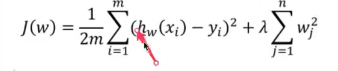
            正则化
                L1
                损失函数 + λ惩罚项
                LASSO
                L2 更常用
                损失函数 + λ惩罚项
                Ridge - 岭回归

4.3 线性回归的改进-岭回归

4.3.1 带有L2正则化的线性回归-岭回归

    alpha 正则化力度=惩罚项系数

损失函数
岭回归

def linear3():
    """
    岭回归对波士顿房价进行预测
    :return:
    """
    # 1）获取数据
    boston = load_boston()
    print("特征数量：\n", boston.data.shape)

    # 2）划分数据集
    x_train, x_test, y_train, y_test = train_test_split(boston.data, boston.target, random_state=22)

    # 3）标准化
    transfer = StandardScaler()
    x_train = transfer.fit_transform(x_train)
    x_test = transfer.transform(x_test)

    # 4）预估器
    # estimator = Ridge(alpha=0.5, max_iter=10000)
    # estimator.fit(x_train, y_train)

    # 保存模型
    # joblib.dump(estimator, "my_ridge.pkl")
    # 加载模型
    estimator = joblib.load("my_ridge.pkl")

    # 5）得出模型
    print("岭回归-权重系数为：\n", estimator.coef_)
    print("岭回归-偏置为：\n", estimator.intercept_)

    # 6）模型评估
    y_predict = estimator.predict(x_test)
    print("预测房价：\n", y_predict)
    error = mean_squared_error(y_test, y_predict)
    print("岭回归-均方误差为：\n", error)

    return None

4.2 欠拟合与过拟合

训练集上表现得好，测试集上不好 - 过拟合

4.2.1 什么是过拟合与欠拟合

    欠拟合
        学习到数据的特征过少
        解决：
            增加数据的特征数量
    过拟合
        原始特征过多，存在一些嘈杂特征， 模型过于复杂是因为模型尝试去兼顾各个测试数据点
        解决：
            正则化
                L1
                损失函数 + λ惩罚项
                LASSO
                L2 更常用
                损失函数 + λ惩罚项
                Ridge - 岭回归

4.3 线性回归的改进-岭回归

4.3.1 带有L2正则化的线性回归-岭回归

    alpha 正则化力度=惩罚项系数

4.4 分类算法-逻辑回归与二分类

4.4.1 逻辑回归的应用场景

    广告点击率 是否会被点击
    是否为垃圾邮件
    是否患病
    是否为金融诈骗
    是否为虚假账号
    正例 / 反例

4.4.2 逻辑回归的原理

    线型回归的输出 就是 逻辑回归 的 输入
    激活函数
        sigmoid函数 [0, 1]
        1/(1 + e^(-x))
    假设函数/线性模型
        1/(1 + e^(-(w1x1 + w2x2 + w3x3 + …… + wnxn + b)))
    损失函数
        (y_predict - y_true)平方和/总数
        逻辑回归的真实值/预测值 是否属于某个类别
        对数似然损失
        log 2 x
    优化损失
        梯度下降

4.4.4 案例：癌症分类预测-良／恶性乳腺癌肿瘤预测

    恶性 - 正例
    流程分析：
        1）获取数据
            读取的时候加上names
        2）数据处理
            处理缺失值
        3）数据集划分
        4）特征工程：
            无量纲化处理-标准化
        5）逻辑回归预估器
        6）模型评估
真的患癌症的，能够被检查出来的概率 - 召回率

4.4.5 分类的评估方法

    1 精确率与召回率
        1 混淆矩阵
            TP = True Possitive
            FN = False Negative
        2 精确率(Precision)与召回率(Recall)
            精确率
            召回率 查得全不全
            工厂 质量检测 次品 召回率
        3 F1-score 模型的稳健型
   总共有100个人，如果99个样本癌症，1个样本非癌症 - 样本不均衡
   不管怎样我全都预测正例(默认癌症为正例) - 不负责任的模型
       准确率：99%
       召回率：99/99 = 100%
       精确率：99%
       F1-score: 2*99%/ 199% = 99.497%
       AUC:0.5
            TPR = 100%
            FPR = 1 / 1 = 100%
   2 ROC曲线与AUC指标
        1 知道TPR与FPR
            TPR = TP / (TP + FN) - 召回率
                所有真实类别为1的样本中，预测类别为1的比例
            FPR = FP / (FP + TN)
                所有真实类别为0的样本中，预测类别为1的比例

#!/usr/bin/env python
# coding: utf-8

# In[1]:


import pandas as pd
import numpy as np


# In[2]:


# 1、读取数据
path = "https://archive.ics.uci.edu/ml/machine-learning-databases/breast-cancer-wisconsin/breast-cancer-wisconsin.data"
column_name = ['Sample code number', 'Clump Thickness', 'Uniformity of Cell Size', 'Uniformity of Cell Shape',
                   'Marginal Adhesion', 'Single Epithelial Cell Size', 'Bare Nuclei', 'Bland Chromatin',
                   'Normal Nucleoli', 'Mitoses', 'Class']

data = pd.read_csv(path, names=column_name)


# In[4]:


data.head()


# In[7]:


# 2、缺失值处理
# 1）替换-》np.nan
data = data.replace(to_replace="?", value=np.nan)
# 2）删除缺失样本
data.dropna(inplace=True)


# In[9]:


data.isnull().any() # 不存在缺失值


# In[10]:


# 3、划分数据集
from sklearn.model_selection import train_test_split


# In[11]:


data.head()


# In[12]:


# 筛选特征值和目标值
x = data.iloc[:, 1:-1]
y = data["Class"]


# In[14]:


x.head()


# In[16]:


y.head()


# In[17]:


x_train, x_test, y_train, y_test = train_test_split(x, y)


# In[19]:


x_train.head()


# In[20]:


# 4、标准化
from sklearn.preprocessing import StandardScaler


# In[21]:


transfer = StandardScaler()
x_train = transfer.fit_transform(x_train)
x_test = transfer.transform(x_test)


# In[22]:


x_train


# In[23]:


from sklearn.linear_model import LogisticRegression


# In[24]:


# 5、预估器流程
estimator = LogisticRegression()
estimator.fit(x_train, y_train)


# In[25]:


# 逻辑回归的模型参数：回归系数和偏置
estimator.coef_


# In[26]:


estimator.intercept_


# In[27]:


# 6、模型评估
# 方法1：直接比对真实值和预测值
y_predict = estimator.predict(x_test)
print("y_predict:\n", y_predict)
print("直接比对真实值和预测值:\n", y_test == y_predict)

# 方法2：计算准确率
score = estimator.score(x_test, y_test)
print("准确率为：\n", score)


# In[28]:


# 查看精确率、召回率、F1-score
from sklearn.metrics import classification_report


# In[29]:


report = classification_report(y_test, y_predict, labels=[2, 4], target_names=["良性", "恶性"])


# In[31]:


print(report)


# In[33]:


y_test.head()


# In[34]:


# y_true：每个样本的真实类别，必须为0(反例),1(正例)标记
# 将y_test 转换成 0 1
y_true = np.where(y_test > 3, 1, 0)


# In[35]:


y_true


# In[36]:


from sklearn.metrics import roc_auc_score


# In[37]:


roc_auc_score(y_true, y_predict)


# In[ ]:

4.5 模型保存和加载

def linear3():
    """
    岭回归对波士顿房价进行预测
    :return:
    """
    # 1）获取数据
    boston = load_boston()
    print("特征数量：\n", boston.data.shape)

    # 2）划分数据集
    x_train, x_test, y_train, y_test = train_test_split(boston.data, boston.target, random_state=22)

    # 3）标准化
    transfer = StandardScaler()
    x_train = transfer.fit_transform(x_train)
    x_test = transfer.transform(x_test)

    # 4）预估器
    # estimator = Ridge(alpha=0.5, max_iter=10000)
    # estimator.fit(x_train, y_train)

    # 保存模型
    # joblib.dump(estimator, "my_ridge.pkl")
    # 加载模型
    estimator = joblib.load("my_ridge.pkl")

    # 5）得出模型
    print("岭回归-权重系数为：\n", estimator.coef_)
    print("岭回归-偏置为：\n", estimator.intercept_)

    # 6）模型评估
    y_predict = estimator.predict(x_test)
    print("预测房价：\n", y_predict)
    error = mean_squared_error(y_test, y_predict)
    print("岭回归-均方误差为：\n", error)

    return None

### 4.6 无监督学习-K-means算法
####    4.6.1 什么是无监督学习
        没有目标值 - 无监督学习
####    4.6.2 无监督学习包含算法
        聚类
        K-means(K均值聚类)
        降维
        PCA
####    4.6.3 K-means原理
####    4.6.5 案例：k-means对Instacart Market用户聚类
        k = 3
        流程分析：
        降维之后的数据
        1）预估器流程
        2）看结果
        3）模型评估
####    4.6.6 Kmeans性能评估指标
        轮廓系数
        如果b_i>>a_i:趋近于1效果越好，
        b_i<<a_i:趋近于-1，效果不好。
        轮廓系数的值是介于 [-1,1] ，
        越趋近于1代表内聚度和分离度都相对较优。
####    4.6.7 K-means总结
        应用场景：
            没有目标值
            分类

#!/usr/bin/env python
# coding: utf-8

# In[1]:


# 1、获取数据
# 2、合并表
# 3、找到user_id和aisle之间的关系
# 4、PCA降维


# In[2]:


import pandas as pd


# In[3]:


# 1、获取数据
order_products = pd.read_csv("./instacart/order_products__prior.csv")
products = pd.read_csv("./instacart/products.csv")
orders = pd.read_csv("./instacart/orders.csv")
aisles = pd.read_csv("./instacart/aisles.csv")


# In[4]:


# 2、合并表
# order_products__prior.csv：订单与商品信息

# 字段：order_id, product_id, add_to_cart_order, reordered
# products.csv：商品信息
# 字段：product_id, product_name, aisle_id, department_id
# orders.csv：用户的订单信息
# 字段：order_id,user_id,eval_set,order_number,….
# aisles.csv：商品所属具体物品类别
# 字段： aisle_id, aisle

# 合并aisles和products aisle和product_id
tab1 = pd.merge(aisles, products, on=["aisle_id", "aisle_id"])


# In[5]:


tab2 = pd.merge(tab1, order_products, on=["product_id", "product_id"])


# In[6]:


tab3 = pd.merge(tab2, orders, on=["order_id", "order_id"])


# In[7]:


tab3.head()


# In[8]:


# 3、找到user_id和aisle之间的关系
table = pd.crosstab(tab3["user_id"], tab3["aisle"])


# In[9]:


data = table[:10000]


# In[10]:


# 4、PCA降维
from sklearn.decomposition import PCA


# In[11]:


# 1）实例化一个转换器类
transfer = PCA(n_components=0.95)

# 2）调用fit_transform
data_new = transfer.fit_transform(data)


# In[12]:


data_new.shape


# In[13]:


data_new


# In[14]:


# 预估器流程
from sklearn.cluster import KMeans


# In[15]:


estimator = KMeans(n_clusters=3)
estimator.fit(data_new)


# In[17]:


y_predict = estimator.predict(data_new)


# In[20]:


y_predict[:300]


# In[21]:


# 模型评估-轮廓系数
from sklearn.metrics import silhouette_score


# In[22]:


silhouette_score(data_new, y_predict)


# In[ ]:

可爱的杨一凡

关注

1
点赞
踩
1

收藏

觉得还不错? 一键收藏
0
评论
机器学习回归与聚类算法

机器学习回归与聚类算法线性回归欠拟合与过拟合岭回归分类算法：逻辑回归模型保存与加载无监督学习 K-means算法4.1 线性回归回归问题：目标值 - 连续型的数据4.1.1 线性回归的原理 2 什么是线性回归函数关系特征值和目标值线型模型线性关系 y = w1x1 + w2x2 + w3x3 + …… + wnxn + b = wTx + b 数据挖掘基础
复制链接

扫一扫