MLP的两种实现（不同在于forward）

import numpy as np
from sklearn import datasets
import matplotlib.pyplot as plt
from matplotlib.colors import ListedColormap
def sigmoid(x):
    return 1 / (1 + np.exp(-x))

def dsigmoid(y):
    return y * (1 - y)

def tanh(x):
    return np.tanh(x)

def dtanh(y):
    return 1.0 - y ** 2

class MLPClassifier:
    def __init__(self, layers, activation='tanh', epochs=20, learning_rate=0.01):
        # 第一层为输入层, 层数应等于样本特征数
        # 最后一层为输出层
        # 再算上中间层, 所以len(layers)最小为3
        self.epochs = epochs
        self.eta = learning_rate
        self.layers = [np.zeros(layers[0])]
        self.weights = []
        self.biases = []
        for i in range(len(layers) - 1):
            # 这三个者的初始值是随意的
            weight = np.random.random((layers[i + 1], layers[i]))
            layer = np.ones(layers[i + 1])
            bias = np.random.random(layers[i + 1])
            self.weights.append(weight)
            self.layers.append(layer)
            self.biases.append(bias)
        if activation == 'tanh':
            self.activation = tanh
            self.dactivation = dtanh
        elif activation == 'sigmoid':
            self.activation = sigmoid
            self.dactivation = dsigmoid
    def fit(self, X, y):
        for _ in range(self.epochs):
            # 随机梯度下降
            indexes = np.random.permutation(X.shape[0])
            for i in range(X.shape[0]):
                self.forward(X[indexes[i]])
                self.backward(y[indexes[i]])
        return self
    # 方便二维图像的可视化, 实际预测的结果可能不止有一个维度, 不一定能和数值进行比较
    def predict(self, X):
        return np.where(self.predict_prob(X) >= 0.5, 1, 0)
    def predict_prob(self, X):
        y = np.empty((X.shape[0], len(self.layers[-1])))
        for i in range(X.shape[0]):
            self.forward(X[i])
            y[i, :] = self.layers[-1]
        return y
    def forward(self, inputs):
        self.layers[0][:] = inputs
        for i in range(len(self.weights)):
            self.layers[i + 1] = self.activation(self.weights[i].dot(self.layers[i]) + self.biases[i])
    def backward(self, y):
        # y 是真实的标签值
        y_predict = self.layers[-1]
        pre_gradient_neurons = y - y_predict  #链式法则
        # 从最后一层到第一层进行遍历, 第0层是输入层, 不在遍历范围内
        for i in range(len(self.layers) - 1, 0, -1):
            gradient_bias = pre_gradient_neurons * self.dactivation(self.layers[i])
            gradient_weight = gradient_bias.reshape(-1, 1).dot(self.layers[i - 1].reshape(1, -1))
            # 先根据当前的 weight 和 gradient_bias 计算下一层的梯度, 再更新weight
            pre_gradient_neurons = gradient_bias.dot(self.weights[i - 1])
            self.weights[i - 1] += self.eta * gradient_weight
            self.biases[i - 1] += self.eta * gradient_bias



def plot_decision_boundary(model, X):
    axis = [np.min(X[:, 0]), np.max(X[:, 0]), np.min(X[:, 1]), np.max(X[:, 1])]
    x0, x1 = np.meshgrid(
        np.linspace(axis[0], axis[1], int((axis[1] - axis[0]) * 100)).reshape(-1, 1),
        np.linspace(axis[2], axis[3], int((axis[3] - axis[2]) * 100)).reshape(-1, 1),
    )
    X_new = np.c_[x0.ravel(), x1.ravel()]
    y_predict = model.predict(X_new)
    zz = y_predict.reshape(x0.shape)
    custom_cmap = ListedColormap(['#EF9A9A', '#FFF59D', '#90CAF9', '#EE82EE', '#00FFFF', '#7FFFAA', '#BDB76B'])
    plt.contourf(x0, x1, zz, cmap=custom_cmap)
if __name__ == '__main__':
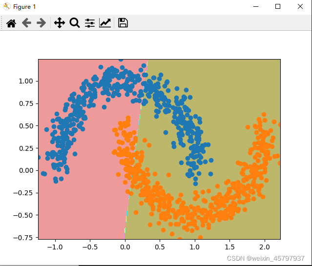
    X, y = datasets.make_moons(n_samples=1000, noise=0.1, random_state=666)
    # 当层数增多时, epochs也应该增多, 不然会欠拟合, 因为要训练的参数增多了
    n = MLPClassifier((2, 3, 1), activation='tanh', epochs=300, learning_rate=0.01)
    n.fit(X, y)
    plot_decision_boundary(n, X)
    plt.scatter(X[y == 0, 0], X[y == 0, 1])
    plt.scatter(X[y == 1, 0], X[y == 1, 1])
    plt.show()

import numpy as np
from sklearn import datasets
import matplotlib.pyplot as plt
from matplotlib.colors import ListedColormap
def sigmoid(x):
    return 1 / (1 + np.exp(-x))
def dsigmoid(y):
    return y * (1 - y)
def tanh(x):
    return np.tanh(x)
def dtanh(y):
    return 1.0 - y ** 2
class MLPClassifier:
    def __init__(self, layers, activation='tanh', epochs=20, batch_size=1, learning_rate=0.01):
        # 第一层为输入层, 层数应等于样本特征数
        # 最后一层为输出层
        # 再算上中间层, 所以len(layers)最小为3
        self.epochs = epochs
        self.eta = learning_rate
        self.batch_size = batch_size
        self.layers = [np.zeros((layers[0], batch_size))]
        self.weights = []
        self.biases = []
        for i in range(len(layers) - 1):
            weight = np.random.random((layers[i + 1], layers[i]))
            layer = np.ones((layers[i + 1], batch_size))
            bias = np.random.random((layers[i + 1], 1))
            self.weights.append(weight)
            self.layers.append(layer)
            self.biases.append(bias)
        if activation == 'tanh':
            self.activation = tanh
            self.dactivation = dtanh
        elif activation == 'sigmoid':
            self.activation = sigmoid
            self.dactivation = dsigmoid
    def fit(self, X, y):
        # 如果y有多个维度的话, y的每一列为一个真实的标签
        if y.ndim == 2:
            assert y.shape[1] == X.shape[0], "each column of y is a label of a row in X"
        for _ in range(self.epochs):
            indexes = np.random.permutation(X.shape[0])
            for i in range(X.shape[0] // self.batch_size):
                start_index = i * self.batch_size
                end_index = start_index + self.batch_size
                self.forward(X[indexes[start_index:end_index]])
                self.backward(y[indexes[start_index:end_index]])
        return self
    def predict(self, X):
        return np.where(self.predict_prob(X) >= 0.5, 1, 0)
    def predict_prob(self, X):
        # 优化了predict函数, 进行向量化处理
        self.forward(X)
        y = self.layers[-1].copy()
        return y
    def forward(self, inputs):
        self.layers[0] = inputs.T
        for i in range(len(self.weights)):
            self.layers[i + 1] = self.activation(self.weights[i].dot(self.layers[i]) + self.biases[i])
    def backward(self, y):#基于小批量梯度下降实现
        # y 是真实的标签值
        y_predict = self.layers[-1]
        pre_gradient_neurons = y - y_predict
        # 从最后一层到第一层进行遍历, 第0层是输入层, 不在遍历范围内
        for i in range(len(self.layers) - 1, 0, -1):
            # 对每一个样本计算bias, weight, neurons的梯度, 再求均值做为最后的梯度
            gradient_bias_matrix = pre_gradient_neurons * self.dactivation(self.layers[i])
            gradient_weight = gradient_bias_matrix.dot(self.layers[i - 1].T) / self.batch_size
            pre_gradient_neurons = np.sum(gradient_bias_matrix.T.dot(self.weights[i - 1]), axis=0) \
                .reshape(-1, 1) / self.batch_size
            # 此时weight和neurons的梯度依赖与bias的梯度矩阵, 而不是平均梯度, 所以最后求bias的平均梯度
            gradient_bias = np.mean(gradient_bias_matrix, axis=1).reshape(-1, 1)
            self.weights[i - 1] += self.eta * gradient_weight
            self.biases[i - 1] += self.eta * gradient_bias

def plot_decision_boundary(model, X):
    axis = [np.min(X[:, 0]), np.max(X[:, 0]), np.min(X[:, 1]), np.max(X[:, 1])]
    x0, x1 = np.meshgrid(
        np.linspace(axis[0], axis[1], int((axis[1] - axis[0]) * 100)).reshape(-1, 1),
        np.linspace(axis[2], axis[3], int((axis[3] - axis[2]) * 100)).reshape(-1, 1),
    )
    X_new = np.c_[x0.ravel(), x1.ravel()]
    y_predict = model.predict(X_new)
    zz = y_predict.reshape(x0.shape)
    custom_cmap = ListedColormap(['#EF9A9A', '#FFF59D', '#90CAF9', '#EE82EE', '#00FFFF', '#7FFFAA', '#BDB76B'])
    plt.contourf(x0, x1, zz, cmap=custom_cmap)
if __name__ == '__main__':
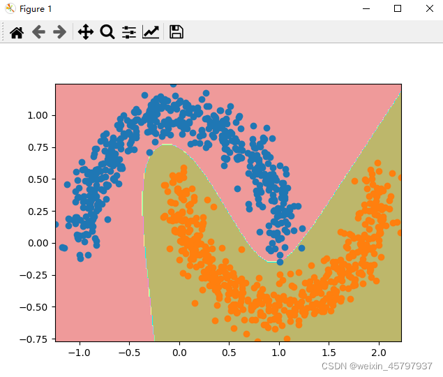
    X, y = datasets.make_moons(n_samples=1000, noise=0.1, random_state=666)
    # 当层数增多时, epochs也应该增多, 不然会欠拟合, 因为要训练的参数增多了
    n = MLPClassifier((2, 3, 1), activation='tanh', epochs=300, learning_rate=0.01)
    n.fit(X, y)
    plot_decision_boundary(n, X)
    plt.scatter(X[y == 0, 0], X[y == 0, 1])
    plt.scatter(X[y == 1, 0], X[y == 1, 1])
    plt.show()