逻辑回归处理数据分类

import  numpy as np
import pandas as pd
import matplotlib.pyplot as plt
import  matplotlib as mpl
import matplotlib.patches as mpaches
%matplotlib inline
from  sklearn.pipeline  import Pipeline
from  sklearn.neighbors  import KNeighborsClassifier
from  sklearn.linear_model  import  LogisticRegression #逻辑回归
from  sklearn.preprocessing  import StandardScaler,PolynomialFeatures

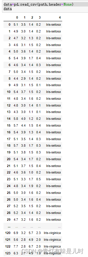
path=r"C:\Users\Tsinghua-yincheng\Desktop\SZday94\data\iris.data"
data=pd.read_csv(path,header=None)
data

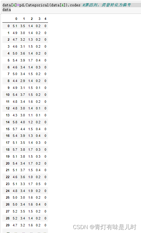
data[4]=pd.Categorical(data[4]).codes #第四列，类型转化为编号
data

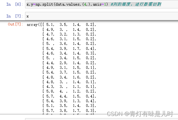
x,y=np.split(data.values,(4,),axis=1) #列的维度，进行数据切割
x
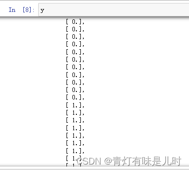
y

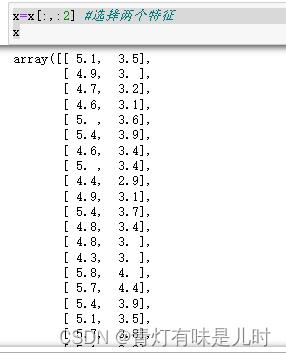
x=x[:,:2] #选择两个特征
x

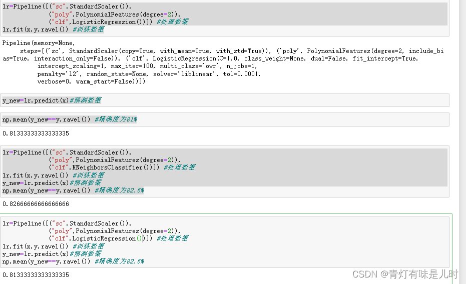
lr=Pipeline([("sc",StandardScaler()),
             ("poly",PolynomialFeatures(degree=2)),
             ("clf",LogisticRegression())]) #处理数据
lr.fit(x,y.ravel()) #训练数据
y_new=lr.predict(x)#预测数据
np.mean(y_new==y.ravel()) #精确度为81%

lr=Pipeline([("sc",StandardScaler()),
             ("poly",PolynomialFeatures(degree=2)),
             ("clf",KNeighborsClassifier())]) #处理数据
lr.fit(x,y.ravel()) #训练数据
y_new=lr.predict(x)#预测数据
np.mean(y_new==y.ravel()) #精确度为82.6%

lr=Pipeline([("sc",StandardScaler()),
             ("poly",PolynomialFeatures(degree=2)),
             ("clf",LogisticRegression())]) #处理数据
lr.fit(x,y.ravel()) #训练数据
y_new=lr.predict(x)#预测数据
np.mean(y_new==y.ravel()) #精确度为82.6%

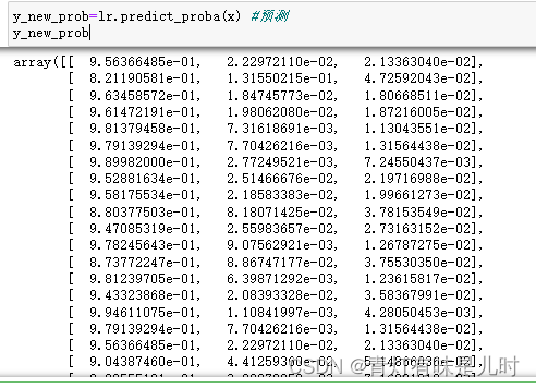
y_new_prob=lr.predict_proba(x) #预测
y_new_prob

#绘图
N,M=500,500#横纵数据采样
x1_min,x1_max=x[:,0].min(),x[:,0].max() #第一列的范围
x2_min,x2_max=x[:,1].min(),x[:,1].max() #第2列的范围
t1=np.linspace(x1_min,x1_max,N)
t2=np.linspace(x2_min,x2_max,M) #数据切割500份
x1,x2=np.meshgrid(t1,t2)#生成表格，
x_test=np.stack((x1.flat,x2.flat),axis=1) #测试的点

mpl.rcParams['font.sans-serif'] = ['simHei']
mpl.rcParams['axes.unicode_minus'] = False#中文乱码

#两个颜色列表
cmp_light=mpl.colors.ListedColormap(["#77AABB",
                                     "#7700BB",
                                     "#77AAFF"])
cmp_dark=mpl.colors.ListedColormap(["g","r","b"])

y_new=lr.predict(x_test)#预测数据
y_new=y_new.reshape(x1.shape) #调整形状

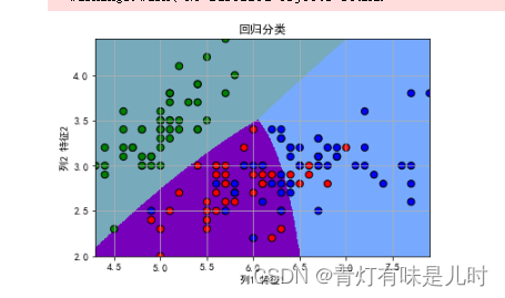
plt.figure(facecolor="w")
plt.pcolormesh(x1,x2,y_new,cmap=cmp_light) #预测的绘图
plt.scatter(x[:,0],x[:,1],c=y,edgecolors="k",s=50,
            cmap=cmp_dark) #绘制样本
plt.xlim(x1_min,x1_max)
plt.ylim(x2_min,x2_max) #设置边界
plt.xlabel("列1 特征1")
plt.ylabel("列2 特征2")
plt.grid()

plt.legend()
plt.title("回归分类")
plt.show()