


文章目录
基本原理
**
Plot = data + mapping +geometry + (Statistics, Scale, Coordinate) + Details
**
Plot: 图形
data:原始数据
mapping:映射
geometry:几何对象(柱状,点,线等)
Statistics:统计分析
Scale:几何元素赋值(如点、颜色和形状等)
Coordinate:坐标系(笛卡尔坐标系、极坐标系等)
Details:作图细节(主题、坐标轴、字体、文字注释等)
基础代码
ggplot2::ggplot(data, aes())+ ## 基础函数 指明数据、x、y及其他映射对象(颜色、填充、形状、透明度)
geom_(aes())+   ## 不同几何图形的映射(点图、柱状图、折线图等)
geom_(aes())+   ## 一般用于添加误差线或者添加其他组合图形
geom_(aes())+
...
scale_()+       ## 将颜色、形状、填充等几何要素指明具体的数据值和形状颜色大小
theme()         ## 修改具体的坐标轴、字体、图例等
常用图
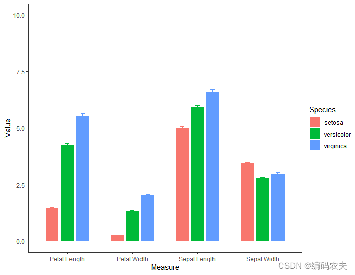
条形图
library(tidyverse)

theme_set(theme_test())
library(sciplot)
iris%>%gather(key=Measure,value="value",-Species)%>%group_by(Species,Measure)%>%
  summarise(mean=mean(value),se=se(value))%>%
  ggplot(aes(x=Measure,y=mean,fill=Species))+
  geom_col(position = position_dodge(0.7),width = 0.6)+
  geom_errorbar(aes(ymin=mean-se,ymax=mean+se,color=Species),position = position_dodge(0.7),width=0.2,size=1)+
  ylim(0,10)+
  labs(y="Value")
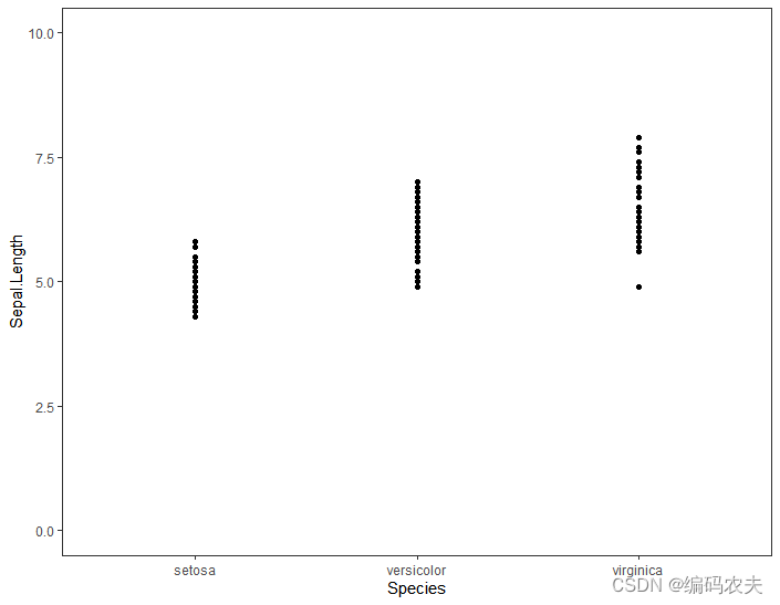
点图
library(tidyverse)

theme_set(theme_test())
iris%>%
  ggplot(aes(x=Species,y=Sepal.Length),fill = "red",color="white")+
  geom_point(color="black",fill="white")+
  ylim(0,10)+
  labs(y="Sepal.Length")
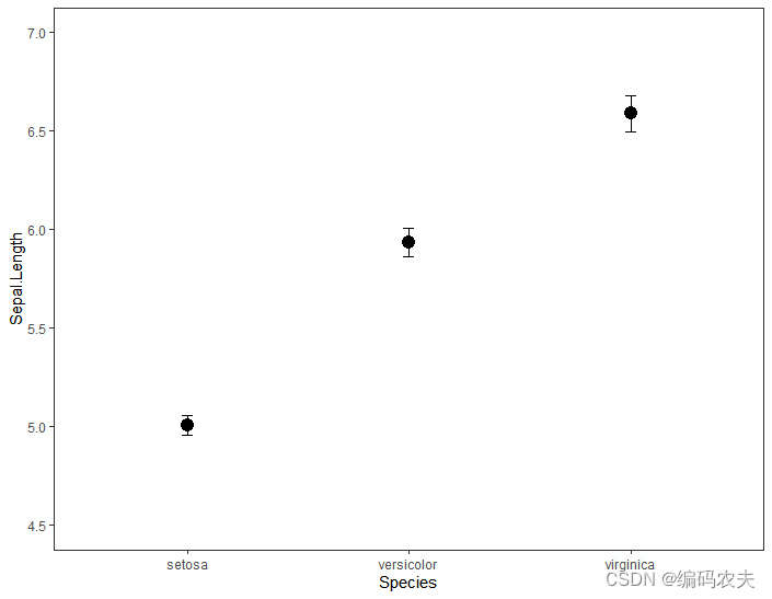
误差线点图
library(tidyverse)

theme_set(theme_test())
library(sciplot)
iris%>%group_by(Species)%>%summarise(mean=mean(Sepal.Length),se=se(Sepal.Length))%>%
  ggplot(aes(x=Species,y=mean),fill = "red",color="white")+
  geom_point(color="black",size=4)+
  geom_errorbar(aes(ymin=mean-se,ymax=mean+se),width=0.05)+
  ylim(4.5,7)+
  labs(y="Sepal.Length")
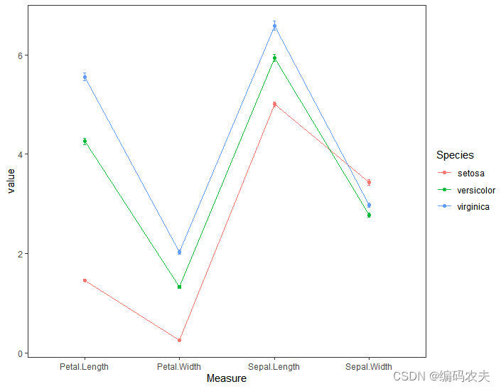
折线图
library(tidyverse)

theme_set(theme_test())
library(sciplot)
iris%>%gather(key=Measure,value="value",-Species)%>%group_by(Species,Measure)%>%
  summarise(mean=mean(value),se=se(value))%>%
  ggplot(aes(x=Measure,y=mean,fill=Species))+
  geom_point(aes(x=Measure,y=mean,color=Species),position = position_dodge(0))+
  geom_line(aes(x=Measure,y=mean,color=Species,group=Species))+
  geom_errorbar(aes(ymin=mean-se,ymax=mean+se,color=Species),position = position_dodge(0),width=0.1)+
  #ylim(4.5,7)+
  labs(y="value")
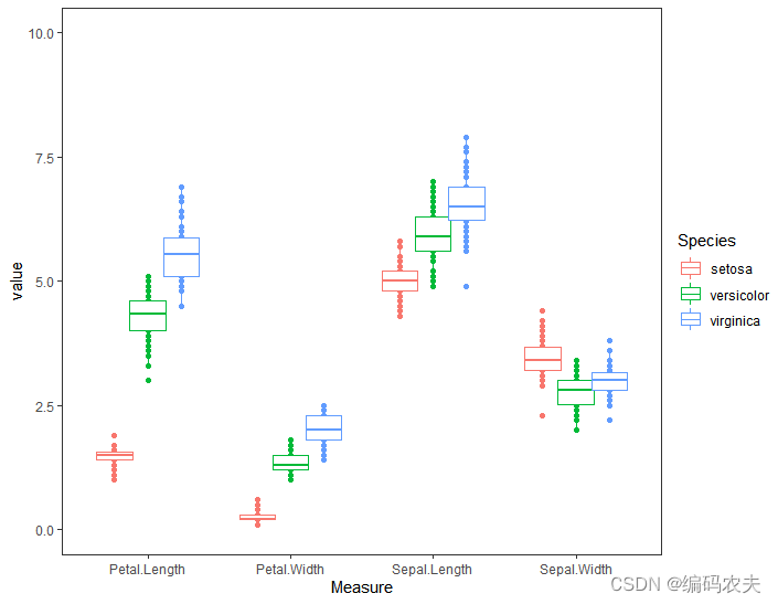
箱线图
library(tidyverse)

theme_set(theme_test())
library(sciplot)
iris%>%gather(key=Measure,value="value",-Species)%>%
  ggplot(aes(x=Measure,y=value,color=Species))+
  geom_point(position = position_dodge(0.7))+
  geom_boxplot(position = position_dodge(0.7))+
  ylim(0,10)+
  labs(y="value")
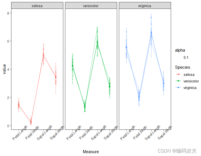
分组配对点图
library(tidyverse)

theme_set(theme_test())
library(sciplot)
iris2 <- iris%>%gather(key=Measure,value="value",-Species)
iris%>%gather(key=Measure,value="value",-Species)%>%group_by(Species,Measure)%>%
  summarise(mean=mean(value),se=se(value))%>%
  ggplot()+
  geom_point(aes(x=Measure,y=mean,color=Species),position = position_dodge(0))+
  geom_line(aes(x=Measure,y=mean,color=Species,group=Species))+
  #geom_errorbar(aes(ymin=mean-se,ymax=mean+se,color=Species),position = position_dodge(0),width=0.1)+
  geom_point(data=iris2,aes(x=Measure,y=value,color=Species),alpha=0.1,position = position_dodge(0))+
  geom_line(data=iris2,aes(x=Measure,y=value,color=Species,alpha=0.1,group=Species))+
  #ylim(4.5,7)+
  facet_grid(~Species,scales = "free")+
  labs(y="value")+
  theme(axis.text.x =  element_text(angle = 45))
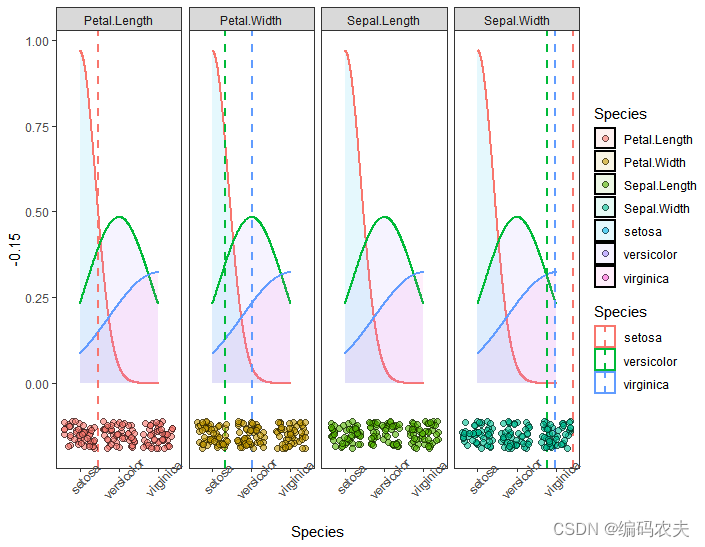
密度图
library(tidyverse)

theme_set(theme_test())
library(sciplot)
iris2 <- iris%>%gather(key=Measure,value="value",-Species)%>%group_by(Species,Measure)%>%
  summarise(mean=mean(value),se=se(value))

iris%>%gather(key=Measure,value="value",-Species)%>%group_by(Species,Measure)%>%
  ggplot()+
  geom_density(aes(x = Species,fill = Species,color = Species),alpha = 0.1,size = 0.75)+
  geom_vline(data=iris2,aes(xintercept = mean,color = Species),size = 0.75,linetype = 2)+
  geom_jitter(aes(x = Species,y = -0.15,fill = Measure),shape = 21,size = 2,alpha = 0.6,height = 0.04)+
  facet_grid(~Measure,scales = "free")+
  theme(axis.text.x =  element_text(angle = 45))
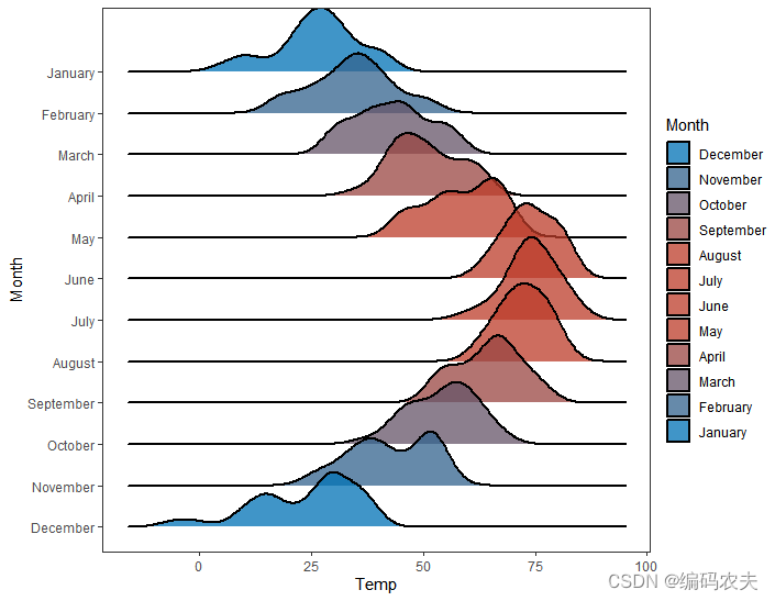
岭图
library(tidyverse)

theme_set(theme_test())
library(sciplot)
library(ggridges)

lincoln_data <- lincoln_weather %>% select("Mean Temperature [F]",Month) %>% rename(Temp = "Mean Temperature [F]")

col <- colorRampPalette(
  c("#0072B5FF","#BC3C29FF","#BC3C29FF","#0072B5FF"))

lincoln_data%>%ggplot()+
  geom_density_ridges(aes(x = Temp,y = Month,fill = Month),scale = 2,size = 0.75,alpha = 0.75)+
  fill_palette(palette = col(12))
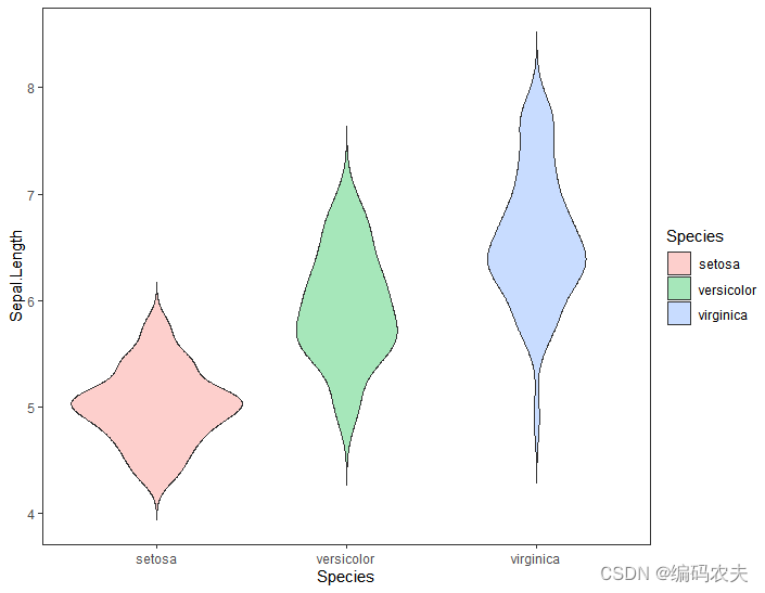
小提琴图
library(tidyverse)

theme_set(theme_test())
iris%>%ggplot()+
  geom_violin(aes(x = Species,y = Sepal.Length,fill = Species),trim = F,alpha = 0.35,size = 0.5)
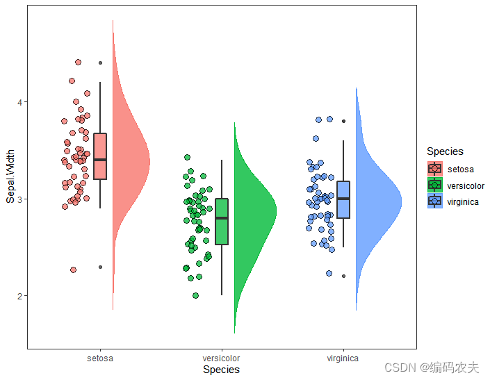
云雨图
library(tidyverse)

theme_set(theme_test())
library(gghalves)
ggplot(data = iris)+
  geom_half_violin(aes(x = Species,y = Sepal.Width,fill = Species,color = Species),side = "r",alpha = 0.8,trim = F,adjust = 1.5,position = position_nudge(x = 0.1))+
  geom_boxplot(aes(x = Species,y = Sepal.Width,fill = Species),width = 0.1,alpha = 0.75,size = 0.8,position = position_dodge(0.75))+
  geom_point(aes(x = as.numeric(Species)-0.2,y = Sepal.Width,fill = Species),shape = 21,size = 3,alpha = 0.75,position = position_jitter(width = 0.1))
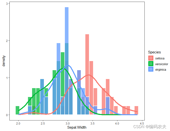
直方图
library(tidyverse)

theme_set(theme_test())
iris%>%select(Species,Sepal.Width)%>%ggplot()+
  geom_histogram(aes(x = Sepal.Width,y = ..density..,fill = Species,color = Species),
                 color = "white",alpha = 0.75,size = 0.75,position = "identity")+
  geom_density(aes(x = Sepal.Width,color = Species),fill = NA,size = 1.5)
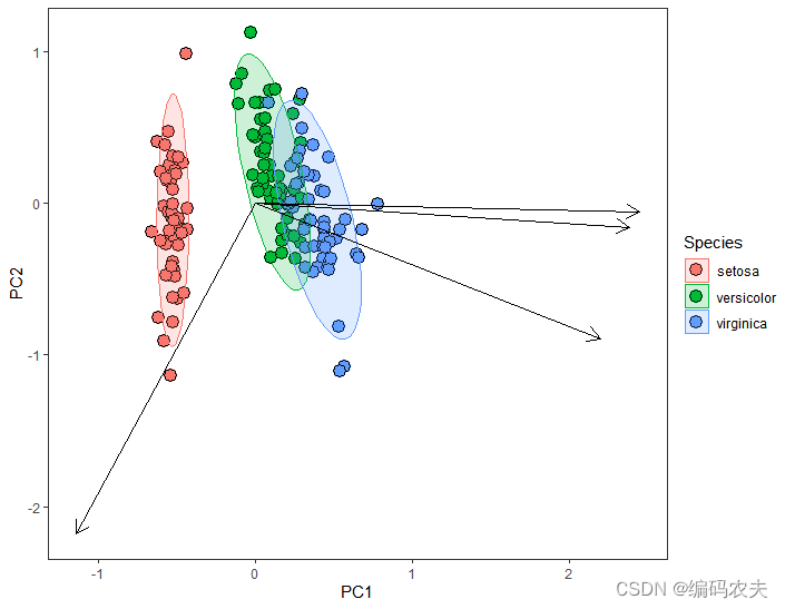
PCA图
library(tidyverse)

theme_set(theme_test())
library(vegan)
pca.data <- iris %>% mutate(Sepal.Length = scale(Sepal.Length),
                            Sepal.Width = scale(Sepal.Width),
                            Petal.Length = scale(Petal.Length),
                            Petal.Width = scale(Petal.Width))
pca <- rda(pca.data[,1:4])
pca.summary <- summary(pca)
pca.result <- as.data.frame(pca.summary$sites) %>% select(-PC3,-PC4) %>% mutate(Species = iris$Species)
pca.arrow <- as.data.frame(pca.summary$species) %>% select(-PC3,-PC4)

library(tidyverse)
pca.result%>%ggplot()+
  geom_point(aes(x = PC1,y = PC2,fill = Species),shape = 21,size = 4)+
  stat_ellipse(aes(x = PC1,y = PC2,color = Species,fill = Species),
               geom ="polygon",level = 0.95,size = 0.5,alpha = 0.2)+
  geom_segment(data = pca.arrow,aes(x = 0,xend = PC1,y = 0,yend = PC2),
               arrow = arrow(length = unit(0.35,"cm")))
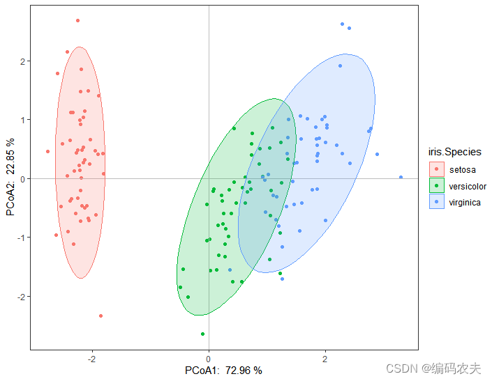
PcoA图
library(tidyverse)

theme_set(theme_test())
library(ape)

library(ade4)

pcoa.data <- iris %>% mutate(Sepal.Length = scale(Sepal.Length),
                             Sepal.Width = scale(Sepal.Width),
                             Petal.Length = scale(Petal.Length),
                             Petal.Width = scale(Petal.Width))

tab.dist <- dist(pcoa.data[,-5])
pcoa <- pcoa(tab.dist)
pcoa_eig <- pcoa$values

sample_site <- pcoa$vectors%>%as.data.frame()

names(sample_site)[1:2] <- c("x","y")

sample_site <- data.frame(sample_site,iris$Species)

sample_site%>%ggplot()+
  geom_point(aes(x,y,color=iris.Species),size = 1.5)+
  geom_vline(xintercept = 0, color = 'gray', size = 0.4) +
  geom_hline(yintercept = 0, color = 'gray', size = 0.4) +
  stat_ellipse(aes(x,y,color = iris.Species,fill = iris.Species),
               geom ="polygon",level = 0.95,size = 0.5,alpha = 0.2)+
  labs(x = paste('PCoA1: ', round(100 * pcoa_eig[1,2], 2), '%'),
       y = paste('PCoA2: ', round(100 * pcoa_eig[2,2], 2), '%'))
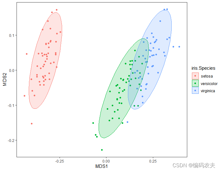
NDMS图
library(tidyverse)

theme_set(theme_test())
library(vegan)

NMDS <- metaMDS(iris[,-5])

NMDS = data.frame(MDS1 = NMDS$points[,1], MDS2 = NMDS$points[,2])

NMDS <- data.frame(NMDS,iris$Species)

NMDS%>%ggplot(aes(MDS1,MDS2))+
  geom_point(aes(MDS1,MDS2,color=iris.Species))+
  stat_ellipse(aes(MDS1,MDS2,color = iris.Species,fill = iris.Species),
               geom ="polygon",level = 0.95,size = 0.5,alpha = 0.2)
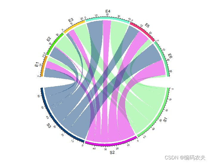
和弦图
library(circlize)

set.seed(999)
mat = matrix(sample(18, 18), 3, 6)
rownames(mat) = paste0("S", 1:3)
colnames(mat) = paste0("E", 1:6)

df = data.frame(from = rep(rownames(mat), times = ncol(mat)),
                to = rep(colnames(mat), each = nrow(mat)),
                value = as.vector(mat),
                stringsAsFactors = FALSE)

chordDiagram(mat)
chordDiagram(df)
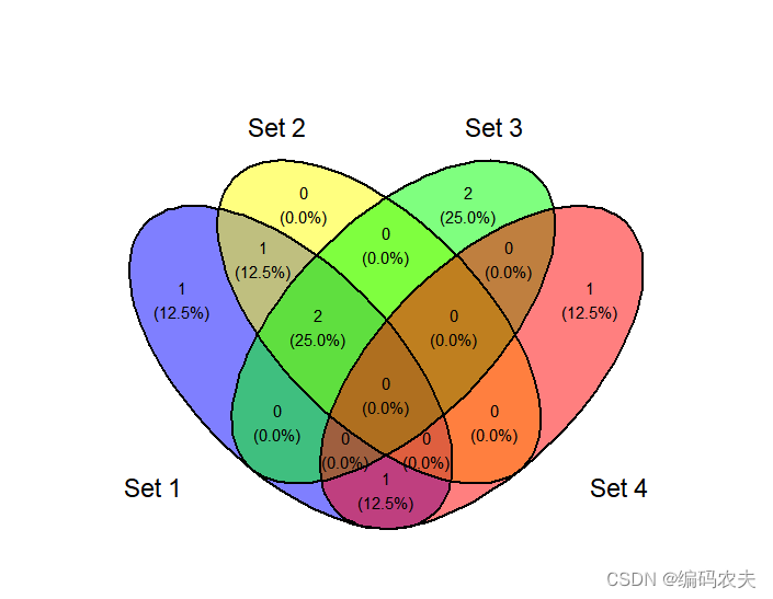
维恩图
library(ggvenn)

d <- tibble(value   = c(1,     2,     3,     5,     6,     7,     8,     9),
            `Set 1` = c(TRUE,  FALSE, TRUE,  TRUE,  FALSE, TRUE,  FALSE, TRUE),
            `Set 2` = c(TRUE,  FALSE, FALSE, TRUE,  FALSE, FALSE, FALSE, TRUE),
            `Set 3` = c(TRUE,  TRUE,  FALSE, FALSE, FALSE, FALSE, TRUE,  TRUE),
            `Set 4` = c(FALSE, FALSE, FALSE, FALSE, TRUE,  TRUE,  FALSE, FALSE))
ggvenn(d, c("Set 1", "Set 2"))
ggvenn(d, c("Set 1", "Set 2", "Set 3"))
ggvenn(d)
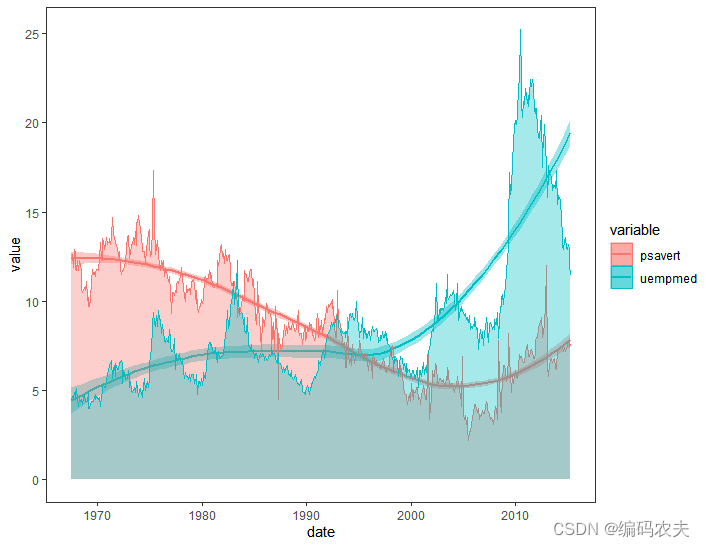
时间序列图
library(tidyverse)

theme_set(theme_test())
time.series.data <- economics %>% select(date,psavert,uempmed) %>%
  gather("psavert","uempmed",key = "variable",value = "value")


ggplot(data = time.series.data ,aes(x = date,y = value,color = variable,fill = variable))+
  geom_line(size = 0.6)+
  geom_smooth()+
  geom_area(alpha = 0.35,position = position_dodge())
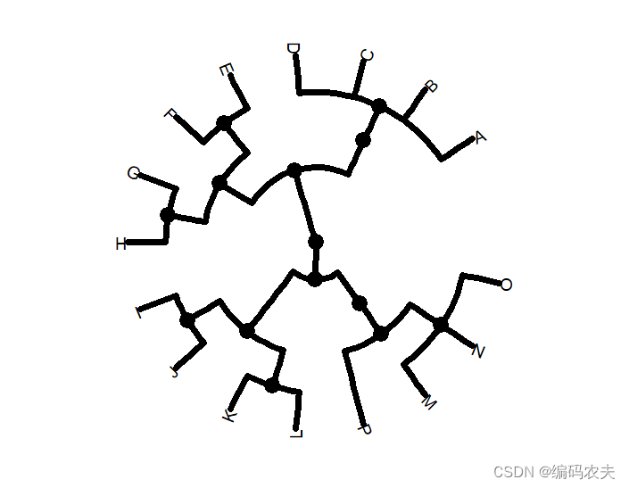
系统发育树
library(ape)
tree <- read.tree(text="((((A,B,C,D)),((E,F),(G,H))),(((I,J),(K,L)),(((M,N,O),P))));")

library(ggtree)
ggtree(tree, branch.length = "none",ladderize = TRUE,size=2) +
  #geom_tiplab(size=5, align=TRUE, linesize=.5,label.offset=1.5) +
  xlim(0,10)

ggtree(tr = tree,layout="circular")+##### branch.length = "none")+
       geom_tree(size = 2.5)+
         geom_nodepoint(size = 6)+
         geom_tiplab(size = 5)
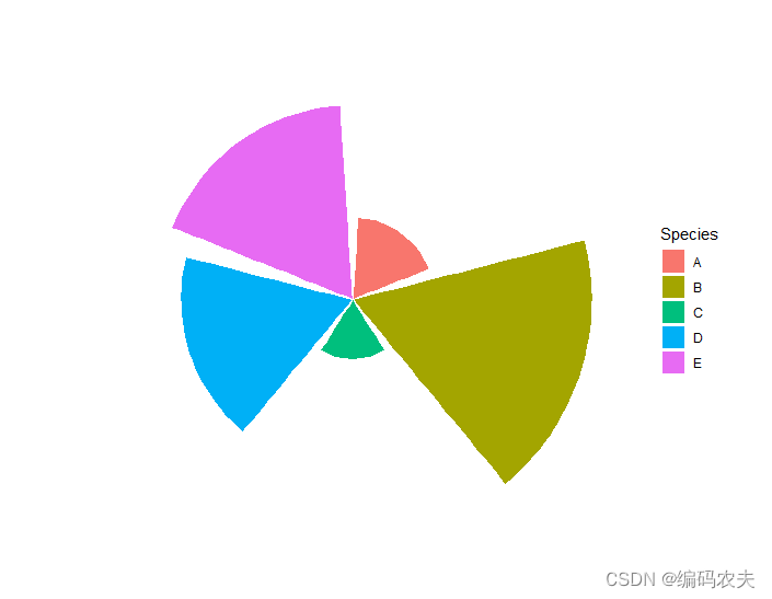
饼图
pie.data <- data.frame(Species = c("A","B","C","D","E"),
                       Prop = c(11,32,8,23,26))

ggplot(data = pie.data,aes(x = Species,y = Prop,fill = Species))+
  geom_bar(stat = "identity",color = "white")+
  coord_polar("x",start = 0,direction = 1)+
  theme_void()
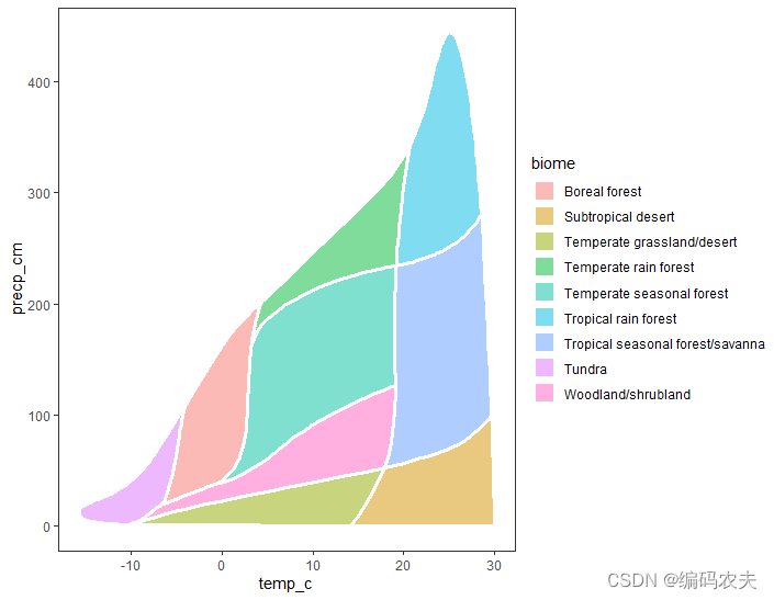
生物区系图
devtools::install_github("valentinitnelav/plotbiomes")
library(plotbiomes)

data(Whittaker_biomes)

Whittaker_biomes%>%ggplot()+
geom_polygon(aes(x = temp_c,y = precp_cm,fill = biome),
             color = "white",size = 1.2,alpha = 0.5)
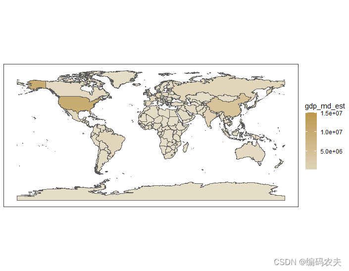
地图
library(sp)
library(ggmap)

library(sf)
library(rnaturalearth)
library(rnaturalearthdata)
library(scatterpie)
library(ggnewscale)

world <- ne_countries(scale = "medium", returnclass = "sf")

ggplot(data = world)+
  geom_sf(aes(fill = gdp_md_est),alpha = 0.8)+
  scale_fill_gradient(low = "#DED4BA",high = "#BC974E")
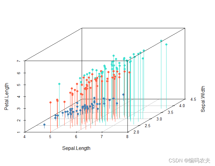
3D图
library(scatterplot3d)

colors <- c("steelblue","tomato","turquoise")
colors <- colors[as.numeric(iris$Species)]

scatterplot3d(iris[,1:3],color = colors,pch = 16,angle = 50,type = "p")
scatterplot3d(iris[,1:3],color = colors,pch = 16,angle = 50,type = "l")
scatterplot3d(iris[,1:3],color = colors,pch = 16,angle = 50,type = "h")
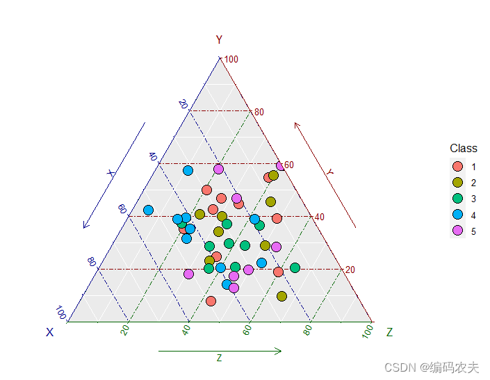
三元图
library(ggtern)

mydata <- data.frame(X = rnorm(50,10,5),Y = rnorm(50,10,5),Z = rnorm(50,10,5),Class = rep(1:5,each = 10)) %>%
  mutate(Class = as.factor(Class))
ggtern(data = mydata,aes(x = X,y = Y,z = Z))+
  geom_point(aes(fill = Class),shape = 21,size = 5)+
  theme_rgbg()
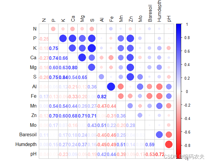
相关性矩阵图
library(corrplot)
library(vegan)

data(varechem)
data(varespec)

res <- cor(varechem)

cols <- colorRampPalette(c("red", "white", "blue"))
corrplot.mixed(res,lower.col = cols(100),upper.col = cols(100),tl.pos="lt",tl.col="black")
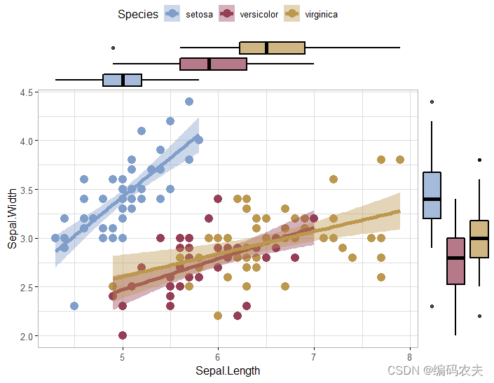
组合图
library(ggpubr)

theme_set(theme_light())


ggscatterhist(data = iris,x = "Sepal.Length",y = "Sepal.Width",shape = 21,size = 4,
              fill = "Species",palette = c("#809ECA","#953F56","#BC974E"),
              margin.params = list(color = "black",size = 1),
              margin.plot = "boxplot",ggtheme = theme_light(),
              add = "reg.line",group = "Species",
              add.params = list(size = 2),conf.int = T)


 653
653


 被折叠的 条评论
为什么被折叠?
被折叠的 条评论
为什么被折叠?
 到【灌水乐园】发言


