Keras基本使用（二）

Savannah913

已于 2022-06-24 10:22:52 修改

阅读量690

点赞数 3

分类专栏：深度学习文章标签：大数据深度学习 keras

于 2022-06-24 09:43:21 首次发布

本文链接：https://blog.csdn.net/weixin_45847320/article/details/125430036

版权

深度学习专栏收录该内容

9 篇文章 0 订阅

订阅专栏

练习一：CNN应用于手写数字识别

Convolution2D进行二维卷积操作，MaxPooling2D：二维的最大池化，Flatten：将数据扁平化一个一维数据

import numpy as np
from keras.datasets import mnist
from keras.utils import np_utils
from keras.models import Sequential
from keras.layers import Dense,Dropout,Convolution2D,MaxPooling2D,Flatten
from keras.optimizers import Adam

#载入数据
(x_train,y_train),(x_test,y_test) = mnist.load_data()
#训练集数据的形状是（6000，28,28），要将训练集数据的形状转换成（6000,28,28,1）
#6000是样本个数，28是图片的长，28是图片的宽，1是图片的深度，（黑白图片深度是1，彩色图片深度是3）
x_train = x_train.reshape(-1,28,28,1)/255.0
#-1是指，给他找一个合适的数，/255.0是进行归一化

#将标签转换为one_hot形式
y_train = np_utils.to_categorical(y_train,num_classes=10)
y_test =np_utils.to_categorical(y_test,num_classes=10)

#定义顺序模型
model = Sequential()

#第一个卷积层
model.add(Convolution2D(
    input_shape = (28,28,1), #输入平面
    filters = 32, #卷积核/滤波器个数
    kernel_size = 5, #卷积窗口大小
    strides = 1, #步长
    padding = "same", #padding方式valid或者same
    activation = "relu" #激活函数
))

#第一个池化层
model.add(MaxPooling2D(
    pool_size = 2,#池化窗口的大小
    strides = 2,
    padding = "same",
))

#第二个卷积层
model.add(Convolution2D(
    filters = 64, #卷积核/滤波器个数
    kernel_size = 5, #卷积窗口大小
    strides = 1, #步长
    padding = "same", #padding方式valid或者same
    activation = "relu" #激活函数
))
#64个特征图，每个特征图大小是14*14

#第二个池化层
model.add(MaxPooling2D(
    pool_size = 2,#池化窗口的大小
    strides = 2,
    padding = "same",
))
#64个特征图，每个特征图大小是7*7

#把第二个池化层的输出扁平化为一维
model.add(Flatten())

#第一个全连接层
model.add(Dense(1024,activation="relu"))#该层有1024个神经元
#Dropout正则化
model.add(Dropout(0.5))
#第二个全连接层,最终的激活函数采用softmax
model.add(Dense(10,activation="softmax"))

#定义优化器
adam = Adam(lr = 1e-4)#学习率为1*10的-4次方

model.compile(optimizer=adam,loss="categorical_crossentropy",metrics=["accuracy"])

#训练模型
model.fit(x_train,y_train,batch_size=64,epochs=10)

#评估模型
loss,accuracy = model.evaluate(x_test,y_test)

print("test loss",loss)
print("test accuracy",accuracy)

显然利用CNN进行图像处理的结果非常好。

练习二：电影评论的二分类问题

加载数据

IMDB数据，50000条严重两级分化的评论，测试集和训练集各占一半，其中，train_data和test_data这两个变量都是评论组成的列表，每条评论是单词索引组成的列表，train_labels和test_labels都是0,1组成的列表，其中0代表负面，1代表正面。

#加载IMDB数据，50000条严重两级分化的评论
from keras.datasets import imdb

(train_data,train_labels),(test_data,test_labels) = imdb.load_data(num_words=10000)
#num=10000表示仅仅保留10000个最常出现的单词，即单词索引不会超过10000
print(train_data[0],train_labels[0])

[1, 14, 22, 16, 43, 530, 973, 1622 ...... 113, 103, 32, 15, 16, 5345, 19, 178, 32] 1

即第一条评论以及其标签。

将某条评论迅速解码为英文单词（补充）

word_index = imdb.get_word_index() #将单词映射为整数索引的字典
print("before\n",list(word_index.items())[:5])

#键值颠倒，将整数索引映射为单词
reverse_word_index = dict(
    [(value,key) for (key,value) in word_index.items()]
)
print("after\n",list(reverse_word_index.items())[:5])

#将评论解码，索引减去3，是因为0,1,2是为填充、序列开始、未知词分别保留的索引
decoded_review = " ".join(
    #dict.get(k,v)
    [reverse_word_index.get(i-3,"?") for i in train_data[0]]
)
print(decoded_review)

dict.get(key,value)，该方法返回字典中键为key的元素对应的值，如果该字典中没有这个键，那么就会返回语句中的value值。

before
 [('fawn', 34701), ('tsukino', 52006), ('nunnery', 52007), ('sonja', 16816), ('vani', 63951)]
after
 [(34701, 'fawn'), (52006, 'tsukino'), (52007, 'nunnery'), (16816, 'sonja'), (63951, 'vani')]
? this film was just brilliant casting location scenery story direction everyone's really suited the part they played and you could just imagine being there robert ? is an amazing actor and now the same being director ? father came from the same scottish island as myself so i loved the fact there was a real connection with this film the witty remarks throughout the film were great it was just brilliant so much that i bought the film as soon as it was released for ? and would recommend it to everyone to watch and the fly fishing was amazing really cried at the end it was so sad and you know what they say if you cry at a film it must have been good and this definitely was also ? to the two little boy's that played the ? of norman and paul they were just brilliant children are often left out of the ? list i think because the stars that play them all grown up are such a big profile for the whole film but these children are amazing and should be praised for what they have done don't you think the whole story was so lovely because it was true and was someone's life after all that was shared with us all

准备数据

不能将整数序列直接输入到神经网络，需要将列表转换为张量，转换方式有两种。

列表转换为张量

方法一： 填充列表，使其具有相同的长度，再将列表转换为形状为(samples, word_indices)的整数张量，然后网络的第一层能够处理这种整数张量的层（Embedding层）。

方法二：对列表进行one_hot编码，转换为只有0,1组成的向量，网络第一层使用Dense层，它能够处理浮点数向量数据。

用第二种方法将列表转换为张量

#将整数序列编码转换为二进制矩阵
import numpy as np
def vectorize_sequences(sequences,dimension=10000):
    results = np.zeros((len(sequences),dimension))
    for i,sequence in enumerate(sequences):
        results[i,sequence] = 1
    return results

#将数据进行向量化
x_train = vectorize_sequences(train_data)
x_test = vectorize_sequences(test_data)

#标签也进行向量化,标签中的数值只有1和0，1表示正面评论，0表示负面评论
y_train = np.asarray(train_labels).astype("float32")
y_test = np.asarray(test_labels).astype("float32")

print("data\n",x_train[:1])
print("labels",y_train)

data
 [[0. 1. 1. ... 0. 0. 0.]]
labels [1. 0. 0. ... 0. 1. 0.]

将数据向量化之后可以输入到标签中了

构建网络

输入数据是向量，标签是只有0,1的标量，这是最简单的情况。解决这种问题采用带有relu激活的全连接层（Dense）的简单堆叠，eg:Dense(16,activation="relu")，16是该层隐藏单元的个数，一个隐藏单元是该层表示空间的一个维度。每个带有relu激活的Dense层都实现了这种向量运算：output = relu(dot(w,input)+b)

16个隐藏单元对应的权重矩阵w的形状为(input_dimension,16)，与w做点积相当于将输入数据投影到16维表示空间中（然后加上偏置b应用relu运算）。

隐藏单元越多（更高维的表示空间），网络越能学到更复杂的表示，网络计算代价也会变得更大，甚至会导致学到不好的模式（这种模式能够提高训练数据上的性能，但是不能提高测试数据的性能）。

对于Dense层的堆叠需要确定两个关键架构：网络有多少层，每层有多少隐藏单元。

此处选择两个中间层，16个隐藏单元进行架构，第三层输出一个标量，预测当前评论的情感。

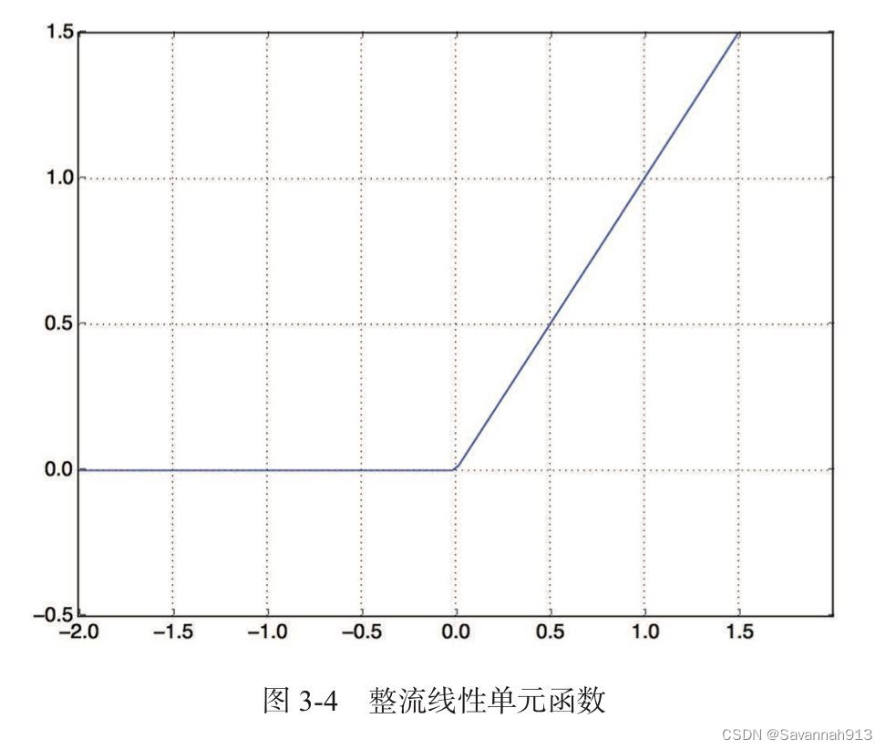
中间层使用relu作为激活函数，最后一层使用sigmoid激活函数输出一个0~1之间的概率值（表示样本目标值等于1的可能性，即评价为正面的可能性），relu函数将所有负值归零，而sigmoid函数则将任意值压缩到[0,1]区间内，其输出值可以看做概率值。

#模型定义
from keros import models
from keros import layers

model = models.Sequential()
model.add(layers.Dense(16,activation="relu",inpur_shape=(10009,)))
model.add(layers.Dense(16,activation="relu"))
model.add(layers.Dense(1,activation="sigmoid"))

模型编译

需要选择损失函数和优化器，由于这是一个二分类问题，网络输出是一个概率值，对于这种概率值的模型，最好使用交叉熵作为loss function，当然也可以使用均方差mse，

#模型编译
model.compile(
    optimizer = "rmsprop",
    loss = "binary_crossentropy",
    metrics = ["accuracy"]
)

上述模型编译是将优化器、损失函数和指标都作为字符串传入，这三个字符串都是Keras内置的一部分，当然也可以自定义优化器、损失函数或者指标函数。

 #配置优化器（自定义损失和指标）
model.compile(
    optimizer = optimizers.RMSprop(lr=0.001),
    loss = 'binary_crossentropy',
    metrics = ['accuracy']
)

进行验证

#留出验证集
x_val = x_train[:10000]
partial_x_train = x_train[10000:]

y_val = y_train[:10000]
partial_y_train = y_train[10000:]

#训练模型
history = model.fit(partial_x_train,partial_y_train,batch_size=520,
                    epochs=10,validation_data=(x_val,y_val))

#评估模型
loss,accuracy = model.evaluate(partial_x_train,partial_y_train)

print("test loss",loss)
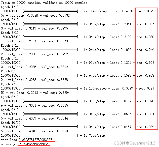
print("accuracy",accuracy)

使用系统配置的优化器运行结果

‘

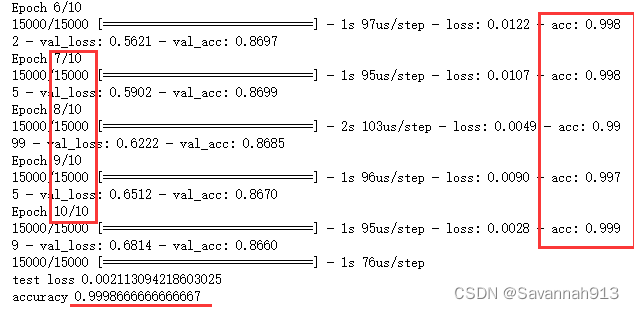
使用自定义损失和指标结果：

显然，自定义优化器和损失之后，精确度提升

绘制损失与精确度

绘制训练集与验证集损失

import matplotlib.pyplot as plt

#绘制训练损失与验证损失
history_dict = history.history
# print(history_dict.keys())     dict_keys(['val_loss', 'val_acc', 'loss', 'acc'])
loss_values = history_dict["loss"]
val_loss_value = history_dict["val_loss"]
_x = range(1, len(loss_values)+1)
plt.plot(_x, loss_values, "r", label="Training loss")
plt.plot(_x, val_loss_values, "b", label="Validation loss")
plt.title("Training and validation loss")
plt.xlabel("Epochs")
plt.ylabel("loss")
plt.legend()
plt.show()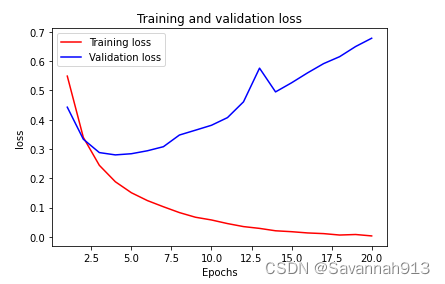

绘制训练精度与验证精度

plt.clf()#清空图像
acc = history_dict["acc"]
val_acc = history_dict["val_acc"]
_x = range(1, len(loss_values)+1)
plt.plot(_x, acc, "r", label="Training acc")
plt.plot(_x, val_acc, "b", label="Validation acc")
plt.title("Training and validation accuracy")
plt.xlabel("Epochs")
plt.ylabel("Accuracy")
plt.legend()
plt.show()

显然，训练损失每轮都在降低，训练精度每轮都在提高，这就是梯度下降优化的预期结果（想让最小化的量随着每次迭代越来越小），显然验证损失和验证精度都并非如此，它们在第四轮差不多达到最佳值。这就是过拟合的情况，即模型在训练数据上表现得非常好，但是在新数据上表现得并不一定越来越好。

为了防止过拟合，可以在第3轮之后停止训练，当然，也可以采用Dropout或者L2正则化的方式来降低过拟合现象。

参数调试

正则化调试

Dropout

model = models.Sequential()
model.add(layers.Dense(16,activation="relu",input_shape=(10000,)))
model.add(Dropout(rate=0.5, input_shape=(10000,)))
model.add(layers.Dense(16,activation="relu"))
model.add(Dropout(rate=0.2))
model.add(layers.Dense(1,activation="sigmoid"))

l2正则化


model = models.Sequential()
model.add(layers.Dense(16,activation="relu",input_shape=(10000,),kernel_regularizer=l2(0.0003)))
model.add(layers.Dense(16,activation="relu",kernel_regularizer=l2(0.0003)))
model.add(layers.Dense(1,activation="sigmoid"))

改变激活函数

relu激活函数

tanh激活函数

显然relu激活函数更胜一筹

以上测试都是基于两个隐藏层

使用三个隐藏层

model = models.Sequential()
model.add(layers.Dense(64,activation="relu",input_shape=(10000,)))
model.add(Dropout(rate=0.5, input_shape=(10000,)))
model.add(layers.Dense(32,activation="relu"))
model.add(Dropout(rate=0.4))
model.add(layers.Dense(16,activation="relu"))
model.add(Dropout(rate=0.2))
model.add(layers.Dense(1,activation="sigmoid"))

且使用自定义优化器！！！（自定义优化器精确率有明显提升）

小结

①通常需要对原始数据进行大量预处理，以便将其转换为张量输入到神经网络中，可以利用one_hot进行二进制编码。

②常用的激活函数relu可以解决包括情感分类在内的很多问题。

③对于二分类问题（两个输出类别），使用sigmoid激活函数（该激活函数常用在二分类问题中，其他问题一般不用），最后一层只有一个单元，表示输出为1的概率（0~1之间）

④二分类问题的sigmoid标量输出，应该使用binary_crossentropy损失函数。

⑤无论你的问题是什么，rmsprop优化器通常是最好的选择！

⑥随着神将网络在训练数据上的表现越来越好，模型最终会过拟合，在新数据上的表现很差，所以一定要监控模型在训练机制外的数据上的性能。

Savannah913

关注

3
点赞
踩
8

收藏

觉得还不错? 一键收藏
0
评论
Keras基本使用（二）

Convolution2D进行二维卷积操作，MaxPooling2D：二维的最大池化，Flatten：将数据扁平化一个一维数据显然利用CNN进行图像处理的结果非常好。 IMDB数据，50000条严重两级分化的评论，测试集和训练集各占一半，其中，train_data和test_data这两个变量都是评论组成的列表，每条评论是单词索引组成的列表，train_labels和test_labels都是0,1组成的列表，其中0代表负面，1代表正面。即第一条评论以及其标签。将某条评论迅速
复制链接

扫一扫