【论文_1992】 REINFORCE » P1 ⭐ 为什么强化学习的目标函数里常看到 log

Williams, R. J. Simple statistical gradient-following algorithms for connectionist reinforcement learning. Mach. Learn., 8:229–256, 1992. PDF 下载链接

——————————————————————————

【REINFORCE_1992_Northeastern University】朴素策略梯度 vanilla policy gradient (also called REINFORCE) (1992) 《Simple Statistical Gradient-Following Algorithms for Connectionist Reinforcement Learning》

https://arxiv.org/abs/1604.06778

REINFORCE (Williams, 1992)： 该算法使用似然比技巧 估计 收益的期望 ${\nabla }_{\theta \eta }({\pi }_{\theta })$ 的梯度:
  ~  
$\widehat{{\nabla }_{\theta \eta }({\pi }_{\theta })}=\frac{1}{NT}\sum _{i=1}^N\sum _{t=0}^T{\nabla }_{\theta }\log \pi (a_t^i|s_t^i;\theta )(R_t^i-b_t^i)$
  ~  
其中 $R_t^i=\sum _{t^{\prime }=t}^T{\gamma }^{t^{\prime }-t}{r}_{t^{\prime }}^i$
$b_t^i$ 是仅依赖于状态 $s_t^i$ 以减少方差的基线。ascent
在估计的梯度方向上采取上升的一步。
这个过程一直持续到 ${\theta }_k$ 收敛。

REINFORCE： 尽管它很简单，但在大多数基本和运动任务中，REINFORCE 是优化深度神经网络策略的有效算法。
即使对于像 Ant 这样的高自由度任务，REINFORCE 也可以获得有竞争力的结果。
然而，我们观察到，正如 Peters 和 Schaal(2008) 指出的那样，REINFORCE 有时会过早收敛到局部最优，这解释了 REINFORCE 和 TNPG 在 Walker 等任务上的表现差距 (图3(a))。
通过对最终策略的可视化，我们可以看到 REINFORCE 的策略结果，这些策略倾向于向前跳跃和摔倒，以最大化短期回报，而不是获得稳定的行走步态以最大化长期回报。
在图 3(b) 中，我们可以观察到，即使在很小的学习率下，REINFORCE 所采取的步骤有时也会导致策略分布的巨大变化，这可以解释快速收敛到局部最优的原因。

——————————————————————————

摘要

This article presents a general class of associative reinforcement learning algorithms for connectionist networks containing stochastic units.
本文提出了一类用于包含随机单元的连接网络的联想强化学习算法。
These algorithms, called REINFORCE algorithms, are shown to make weight adjustments in a direction that lies along the gradient of expected reinforcement in both immediate-reinforcement tasks and certain limited forms of delayed-reinforcement tasks, and they do this without explicitly computing gradient estimates or even storing information from which such estimates could be computed.
这些算法被称为 REINFORCE 算法，在即时强化任务 和 某些有限形式的延迟强化任务中，在沿着预期强化梯度的方向上进行权重调整，并且它们在没有明确计算梯度估计或 甚至存储可以计算这些估计的信息 的情况下这样做。
Specific examples of such algorithms are presented, some of which bear a close relationship to certain existing algorithms while others are novel but potentially interesting in their own right.
提出了这些算法的具体示例，其中一些与某些现有算法有密切的关系，而另一些则是新颖的，但本身可能很有趣。
Also given are results that show how such algorithms can be naturally integrated with backpropagation.
还给出了一些结果，表明这种算法如何自然地与反向传播相结合。
We close with a brief discussion of a number of additional issues surrounding the use of such algorithms, including what is known about their limiting behaviors as well as further considerations that might be used to help develop similar but potentially more powerful reinforcement learning algorithms.
最后，我们简要讨论了围绕此类算法使用的一些其他问题，包括已知的它们的限制行为，以及可能用于帮助开发类似但可能更强大的强化学习算法的进一步考虑。

Keywords. Reinforcement learning, connectionist networks, gradient descent, mathematical analysis
关键词：强化学习，链结式网络，梯度下降，数学分析

1 引言

The general framework of reinforcement learning encompasses a broad variety of problems ranging from various forms of function optimization at one extreme to learning control at the other.
强化学习的一般框架包含了各种各样的问题，从一个极端的各种形式的函数优化 到 另一个极端的学习控制。
While research in these individual areas tends to emphasize different sets of issues in isolation, it is likely that effective reinforcement learning techniques for autonomous agents operating in realistic environments will have to address all of these issues jointly.
这些单独领域的研究 倾向于强调不同问题的孤立集合，但在现实环境中运行的自主代理的有效强化学习技术很可能必须共同解决所有这些问题。
Thus while it remains a useful research strategy to focus on limited forms of reinforcement learning problems simply to keep the problems tractable, it is important to keep in mind that eventual solutions to the most challenging problems will probably require integration of a broad range of applicable techniques.
因此，专注于有限形式的强化学习问题仍然是一种有用的研究策略，只是为了保持问题的可处理性，但重要的是要记住，最具挑战性问题的最终解决方案可能需要集成广泛的适用技术。

In this article we present analytical results concerning certain algorithms for tasks that are associative, meaning that the learner is required to perform an input-output mapping, and, with one limited exception, that involve immediate reinforcement, meaning that the reinforcement (i.e.,payoff) provided to the learner is determined by the most recent input-output pair only.
在本文中，我们给出了关于关联任务的某些算法的分析结果，这意味着学习者learner 需要执行输入-输出映射，并且，除了一个有限的例外，涉及立即强化，这意味着提供给学习者的强化(即回报 payoff )仅由最近的输入-输出对决定。
While delayed reinforcement tasks are obviously important and are receiving much-deserved attention lately, a widely used approach to developing algorithms for such tasks is to combine an immediatere-inforcement learner with an adaptive predictor or critic based on the use of temporal difference methods (Sutton, 1988).
延迟强化任务显然很重要，并且最近受到了非常应得的关注，但针对此类任务开发算法的一种广泛使用的方法是将 即时强化学习器(immediatere-inforcement learner) 与 自适应预测器 或 基于时序差分方法(Sutton, 1988)的 评价者critic 结合起来。
The actor-critic algorithms investigated by Barto, Sutton, and Anderson (1983) and by Sutton (1984) are clearly of this form, as is the Q-learning algorithm of Watkins(1989; Barto, Sutton, & Watkins, 1990).
actor-critic 算法是 Barto、Sutton 和 Anderson(1983) 研究的， Sutton(1984) 的算法显然是这种形式，Watkins 的 Q-learning 算法(1989； Barto, Sutton， & Watkins, 1990) 也是如此。

A further assumption we make here is that the learner’s search behavior, always a necessary component of any form of reinforcement learning algorithm, is provided by means of randomness in the input-output behavior of the learner.
我们在这里做的进一步假设是，学习者的搜索行为，总是任何形式的强化学习算法的必要组成部分，通过学习者输入-输出行为的随机性提供的。
While this is a common way to achieve the desired exploratory behavior, it is worth noting that other strategies are sometimes available in certain cases, including systematic search or consistent selection of the apparent best alternative.
这是实现预期探索行为的常见方法，但值得注意的是，在某些情况下，有时也可以使用其它策略，包括系统搜索或一致选择明显的最佳替代方案。
This latter strategy works in situations where the goodness of alternative actions is determined by estimates which are always overly optimistic and which become more realistic with continued experience, as occurs for example in A* search (Nilsson, 1980).
后一种策略适用于这样的情况，即可择动作的好坏取决于总是过于乐观的估计，并且随着持续的经验而变得更加现实，例如在 A* 搜索中(Nilsson, 1980)。

In addition, all results will be framed here in terms of connectionist networks, and the main focus is on algorithms that follow or estimate a relevant gradient.
此外，所有结果都将在这里以 链结式网络 的形式进行构建，主要关注的是遵循或估计相关梯度的算法。
While such algorithms are known to have a number of limitations, there are a number of reasons why their study can be useful.
First, as experience with backpropagation (leCun, 1985; Parker, 1985; Rumelhart, Hinton, & Williams, 1986; Werbos, 1974) has shown, the gradient seems to provide a powerful and general heuristic basis for generating algorithms which are often simple to implement and surprisingly effective in many cases.
已知这种算法有许多局限性，但有许多原因可以解释为什么它们的研究是有用的：
首先，反向传播(leCun, 1985; Parker, 1985; Rumelhart, Hinton, & Williams, 1986; Werbos, 1974) 的经验表明，梯度似乎为生成算法提供了一个强大而通用的启发式基础，这些算法通常易于实现，并且在许多情况下非常有效。
Second, when more sophisticated algorithms are required, gradient computation can often serve as the core of such algorithms.
其次，当需要更复杂的算法时，梯度计算 通常可以作为这些算法的核心。
Also, to the extent that certain existing algorithms resemble the algorithms arising from such a gradient analysis, our understanding of them may be enhanced.
此外，在某种程度上，某些现有算法类似于 由这种梯度分析产生的算法，我们对它们的理解可能会增强。

Another distinguishing property of the algorithms presented here is that while they can be described roughly as statistically climbing an appropriate gradient, they manage to do this without explicitly computing an estimate of this gradient or even storing information from which such an estimate could be directly computed.
这里提出的算法的另一个显著特性是，它们可以粗略地描述为在统计上攀登一个适当的梯度，但它们设法做到这一点，而不显式地计算这个梯度的估计，或 甚至不存储可以直接计算这种估计的信息。
This is the reason they have been called simple in the title.
Perhaps a more informative adjective would be non-model-based. This point is discussed further in a later section of this paper.
这就是它们在标题中被称为简单的原因。
也许一个更有意义的形容词是非基于模型的。这一点将在本文后面的部分进一步讨论。

Although we adopt a connectionist perspective here, it should be noted that certain aspects of the analysis performed carry over directly to other ways of implementing adaptive input-output mappings.
我们在这里采用了链结式的角度，但应该注意的是，所执行的分析的某些方面直接延续到 实现自适应输入-输出映射的其他方式。
The results to be presented apply in general to any learner whose input-output mapping consists of a parameterized input-controlled distribution function from which outputs are randomly generated, and the corresponding algorithms modify the learner’s distribution function on the basis of performance feedback.
本文的研究结果一般适用于任何学习者，其 输入-输出映射由 参数化的输入控制分布函数 组成，其中随机产生输出，相应的算法根据性能反馈修改学习者的分布函数。
Because of the gradient approach used here, the only restriction on the potential applicability of these results is that certain obvious differentiability conditions must be met.
由于这里使用的是梯度方法，对这些结果的潜在适用性的唯一限制是必须满足某些明显的可微性条件。

A number of the results presented here have appeared in various form in several earlier technical reports and conference papers (Williams, 1986; 1987a; 1987b; 1988a; 1988b).
这里介绍的一些结果以各种形式出现在早期的一些技术报告和会议论文中 (Williams, 1986;1987年;1987 b;1988年;1988 b)。

2 强化学习的链结式网络

除非另有说明，否则我们始终假设学习代理learning agent 是由几个独立单元组成的前馈网络，每个单元本身都是一个学习代理。
我们首先做了一个额外的假设，即所有单元都是随机运行的，但稍后考虑网络中也有确定性单元的情况将是有用的。
网络的运作方式是接收来自环境的外部输入，通过网络传播相应的活动，并将其输出单元产生的活动发送给环境进行评估。
评估由标量增强信号 $r$ 组成，我们假设该信号广播给网络中的所有单元。
此时，每个单元根据所使用的特定 学习算法对其权重进行适当的修改，循环再次开始。

我们自始至终使用的符号如下:
令 $y_i$ 表示网络中第 $i$ 个单元的输出，
${\mathbf{x}}^i$ 表示该单元的输入形式，
输入 ${\mathbf{x}}^i$ 的形式是一个向量，其单个元素(通常表示为 $x_j$ ) 要么是网络中某些单元的输出(那些单元将其输出直接发送到第 $i$ 个单元)，要么是来自环境的某些输入(如果该单元恰好连接在一起，因此它直接接收来自环境的输入)。
输出 $y_i$ 是从依赖于 ${\mathbf{x}}^i$ 的分布和该单元输入线上的权重 $w_{ij}$ 中绘制的。
对于每个 $i$，设 ${\mathbf{w}}^i$ 表示由所有权重 $w_{ij}$ 组成的权重向量。
令 $\mathbf{W}$ 表示由网络中所有权重 $w_{ij}$ 组成的权重矩阵。
在更一般的设置中，${\mathbf{w}}^i$ 可以被视为第 $i$ 个单元(或代理agent )的行为所依赖的所有参数的集合，而 $\mathbf{W}$ 是整个网络(或代理集合)的行为所依赖的参数的集合。

另外，对于每一个 $i$ ，令 g i ( ξ , w i , x i ) = Pr { y i = ξ ∣ w i , x i } g_i(\xi,{\bf w}^i,{\bf x}^i) = {\text {Pr}}\{y_i=\xi |{\bf w}^i,{\bf x}^i\} gi​(ξ,wi,xi)=Pr{yi​=ξ∣wi,xi}，使 $g_i$ 是概率质量函数，确定 $y_i$ 的值是 单元的参数 及 其输入 的函数。
(为了便于说明，我们始终使用适合以下情况的术语和符号：可能的输出值集合 $y_i$ 是离散的，但当取 $g_i$ 为相应的概率密度函数时，导出的结果也适用于连续值单元。)
由于向量 ${\mathbf{w}}^i$ 包含了第 $i$ 个单元的输入输出行为所依赖的所有网络参数，我们也可以定义 g i ( ξ , w i , x i ) = Pr { y i = ξ ∣ W i , x i } g_i(\xi,{\bf w}^i,{\bf x}^i) = {\text {Pr}}\{y_i=\xi |{\bf W}^i,{\bf x}^i\} gi​(ξ,wi,xi)=Pr{yi​=ξ∣Wi,xi}。

请注意，我们在这里命名的许多量，如 $r$, $y_i$ 和 ${\mathbf{x}}^i$，实际上依赖于时间，但在后续中通常可以方便地抑制对这种时间依赖性的显式引用，理解为当几个这样的量出现在单个方程中时，它们代表同一时间步长 $t$ 的值。
我们假设每个新的时间步长都在外部输入呈现给网络之前开始。
在 即时强化任务的背景下，我们也称网络环境相互作用的每个时间步的周期为试验 trial。

为了说明这些定义并引入一个有用的子类，我们定义一个随机半线性单元为 其输出 $y_i$ 是从某个给定的概率分布中得到的，它的质量函数只有一个参数 $p_i$，可以计算为:
  ~  
$p_i=f_i(s_i)(1)$
  ~  
其中 $f_i$ 是一个可微的压缩函数 (squashing function)， 且
  ~  
$s_i={{\mathbf{w}}^i}^T{\mathbf{x}}^i=\sum _j{w}_{ij}{x}_j(2)$
  ~  
${\mathbf{w}}^i$ 和 ${\mathbf{x}}^i$ 的内积。
这可以看作是一个半线性单元，在链结式网络中广泛使用，然后是一个单参数化随机数生成器。

随机半线性单元的一个值得注意的特例是 伯努利半线性单元，其输出 $y_i$ 是一个参数为 $p_i$ 的伯努利随机变量，这意味着唯一可能的输出值是 0 和 1,
Pr { y i = 0 ∣ w i , x i } = 1 − p i {\text {Pr}}\{y_i=0 |{\bf w}^i,{\bf x}^i\}=1-p_i Pr{yi​=0∣wi,xi}=1−pi​
Pr { y i = 1 ∣ w i , x i } = p i {\text {Pr}}\{y_i=1 |{\bf w}^i,{\bf x}^i\}=p_i Pr{yi​=1∣wi,xi}=pi​
因此，对于伯努利半线性单元：
  ~  
$g_i(\xi ,{\mathbf{w}}^i,{\mathbf{x}}^i)=\{\begin{array}{ll}1-p_i& \text{if}\xi =0\\ p_i& \text{if}\xi =1\end{array}$
  ~  
$p_i$ 是通过式 1 和 式 2 计算的。 $p_i=f_i(\sum _j{w}_{ij}{x}_j)$
这种类型的单元在使用随机单元的网络中很常见;
例如，它出现在玻尔兹曼机 (Hinton & Sejnowski, 1986) 和 Barto 及其同事(Barto & Anderson, 1985;Barto & Jordan, 1987;Barto, Sutton， & browwer, 1981) 探索的强化学习网络。
伯努利半线性单元的名称可能看起来只是一个非常熟悉的东西的一个花哨的新名称，使用这个术语是为了强调它在一个潜在的更一般的类中的成员资格。

常用的压缩函数 (squashing function) 的一种特殊形式是对数几率函数 (logistic function)，由
  ~  
$f_i(s_i)=\frac{1}{1+e^{-s_i}}(3)$
  ~  
同时使用伯努利随机数生成器 和 logistic压缩函数的 随机半线性单元称为 Bernoulli-logistic 单元。

现在我们观察到，伯努利半线性单元的类别 包括某些类型的单元，它们的计算可以用线性阈值计算和加性输入噪声或 带噪声阈值 来描述。
这一观察是有用的，因为后一种表述是 Barto 及其同事 (Barto, 1985; Barto & Anandan, 1985; Barto& Anderson, 1985; Barto, Sutton, & Anderson, 1983; Barto, Sutton, & Brouwer, 1981; Sutton,1984) 在他们的研究中使用的。
具体来说，他们假设一个单元通过下式计算它的输出 $y_i$：
  ~  
$y_i=\{\begin{array}{ll}1& \text{if}{\Sigma }_j{w}_{ij}{x}_j+\eta >0\\ 0& \text{otherwise}\end{array}$
  ~  
其中 $\eta$ 是从给定分布 $\Psi$ 中随机抽取的。
为了说明这样的单元可以视为 伯努利半线性单元，设 $s_i={\Sigma }_j{w}_{ij}{x}_j$，观察：
  ~  
Pr { y i = 1 ∣ w i , x i } = Pr { y i = 1 ∣ s i } = Pr { s i + η > 0 ∣ s i }   = 1 − Pr { s i + η ≤ 0 ∣ s i } = 1 − Pr { η ≤ − s i ∣ s i } = 1 − Ψ ( − s i ) \begin{aligned}\text{Pr}\{y_i=1|{\bf w}^i, {\bf x}^i\}&=\text{Pr}\{y_i=1|s_i\}\\ &=\text{Pr}\{s_i+\eta>0|s_i\}\\\ &=1-\text{Pr}\{s_i+\eta\leq0|s_i\}\\ &=1-\text{Pr}\{\eta\leq-s_i|s_i\}\\ &=1-\Psi(-s_i)\end{aligned} Pr{yi​=1∣wi,xi} ​=Pr{yi​=1∣si​}=Pr{si​+η>0∣si​}=1−Pr{si​+η≤0∣si​}=1−Pr{η≤−si​∣si​}=1−Ψ(−si​)​
  ~  
因此，只要 $\Psi$ 是可微的，这个单元就是一个伯努利半线性单位，其压缩函数 $f_i$ 由 $f_i(s_i)=1-\Psi (-s_i)$ 给出。

3 期望强化性能准则

为了考虑梯度学习算法，有必要有一个性能指标来优化。
对于任何即时强化学习问题，无论是否关联，一个非常自然的目标函数是强化信号的期望值，它取决于学习系统的特定参数选择。
因此，对于强化学习网络，我们的性能度量为 E { r ∣ W } E\{r|{\bf W}\} E{r∣W}，
其中 $E$ 表示期望算子，$r$ 表示强化信号，$\mathbf{W}$ 表示网络的权重矩阵。
我们需要在这里使用期望值，因为在以下任何情况下都存在潜在的随机性: 【使用 期望值 的 3 个原因：】
(1) the environment’s choice of input to the network;
环境 给网络 选择的输入 有随机性;
(2) the network’s choice of output corresponding to any particular input;
网络 对任何特定输入 所选择的对应输出 有随机性;
(3) the environment’s choice of reinforcement value for any particular input/output pair.
环境 对任意特定输入/输出对 选择的强化值 有随机性。
请注意，如果我们假设随机性的第一和第三个来源由平稳分布决定，并且环境对网络输入模式的选择也在时间上独立决定，那么独立于时间讨论 E { r ∣ W } E\{r|{\bf W}\} E{r∣W} 是有意义的。
在没有这些假设的情况下，任何给定时间步长的期望值 $r$ 可能是时间的函数，也可能是系统历史的函数。
因此，我们自始至终默认这些平稳性和独立性条件成立。

请注意，在这些假设下， E { r ∣ W } E\{r|{\bf W}\} E{r∣W} 是 $\mathbf{W}$ 的一个定义良好的确定性函数(但对于学习系统来说是未知的)。
因此，在这个公式中，强化学习系统的目标是在所有可能的权重矩阵 $\mathbf{W}$ 的空间中搜索 E { r ∣ W } E\{r|{\bf W}\} E{r∣W} 最大的点。

4 REINFORCE 算法

考虑一个面向一个关联的即时强化学习任务 的网络。
回想一下，在每次试验trial 收到强化值 $r$ 后，在该网络中调整权重。
假设这个网络的学习算法是这样的，在每次试验trial 结束时，网络中的每个参数 $w_{ij}$ 都增加一个量
  ~  
$\Delta w_{ij}={\alpha }_{ij}(r-b_{ij})e_{ij}$
  ~  
其中 ${\alpha }_{ij}$ 为学习率因子，
$b_{ij}$ 为强化基线，
$e_{ij}=\frac{\partial \ln g_i}{\partial w_{ij}}$ 称为 $w_{ij}$ 的 特征合格性characteristic eligibility。
进一步假设强化基线 $b_{ij}$ 条件独立于 $y_i$，在给定 $\mathbf{W}$ 和 $\mathbf{x}$ 的情况下，速率因子 ${\alpha }_{ij}$ 非负且最多依赖于 ${\mathbf{w}}^i$ 和 $t$ (通常将 ${\alpha }_{ij}$ 取为常数)。
任何具有这种特殊形式的学习算法都被称为 REINFORCE 算法。
这个名字是 “REward Increment = Nonnegative Factor times Offset Reinforcement times Characteristic Eligibility,” 的首字母缩略词，它描述了算法的形式。

这类算法的有趣之处在于以下数学结果:

定理 1： 对于任何 REINFORCE 算法， E { Δ W ∣ W } E\{\Delta {\bf W}|{\bf W}\} E{ΔW∣W} 和 ∇ w E { r ∣ W } \nabla _{\bf w}E\{r|{\bf W}\} ∇w​E{r∣W} 的内积是非负的。 即 E { Δ W ∣ W } T ∇ w E { r ∣ W } ≥ 0 E\{\Delta {\bf W}|{\bf W}\}^T\nabla _{\bf w}E\{r|{\bf W}\} ≥ 0 E{ΔW∣W}T∇w​E{r∣W}≥0
更进一步，如果对所有 $i$ 和 $j$， 都有 ${\alpha }_{ij}$ > 0，那么只有当 ∇ w E { r ∣ W } = 0 \nabla _{\bf w}E\{r|{\bf W}\}=0 ∇w​E{r∣W}=0 时，这个内积才为 0。
同样，如果 ${\alpha }_{ij}=\alpha$ 独立于 $i$ 和 $j$，则 E { Δ W ∣ W } = α ∇ w E { r ∣ W } E\{\Delta {\bf W}|{\bf W}\} = \alpha \nabla _{\bf w}E\{r|{\bf W}\} E{ΔW∣W}=α∇w​E{r∣W}。

该结果将任意 REINFORCE 算法的性能度量 E { r ∣ W } E\{r|{\bf W}\} E{r∣W} 在权重空间中的梯度 ∇ w E { r ∣ W } \nabla _{\bf w}E\{r|{\bf W}\} ∇w​E{r∣W} 与 权重空间中的平均更新向量 E { Δ W ∣ W } E\{\Delta {\bf W}|{\bf W}\} E{ΔW∣W} 联系起来。

• 更详细地说， ∇ w E { r ∣ W } \nabla _{\bf w}E\{r|{\bf W}\} ∇w​E{r∣W} 和 E { Δ W ∣ W } E\{\Delta {\bf W}|{\bf W}\} E{ΔW∣W} 都是与 $\mathbf{W}$ 具有相同维数的向量，
  其中 ∇ w E { r ∣ W } \nabla _{\bf w}E\{r|{\bf W}\} ∇w​E{r∣W} 在坐标 $(i,j)$ 处的值为 ∂ E { r ∣ W } ∂ w i j \frac{\partial E\{r|{\bf W}\}}{\partial w_{ij}} ∂wij​∂E{r∣W}​;
  E { Δ W ∣ W } E\{\Delta {\bf W}|{\bf W}\} E{ΔW∣W} 在坐标 $(i,j)$ 处的值为 E { Δ w i j ∣ W } E\{\Delta w_{ij}| {\bf W}\} E{Δwij​∣W}。

具体来说，它表示对于任何这样的算法，权重空间中的平均更新向量位于该性能度量增加的方向。
该定理的最后一句话等价于这样的声明： 对于每个权重 $w_{ij}$，量 $(r-b_{ij})\frac{\partial \ln g_i}{\partial w_{ij}}$ 表示 ∂ E { r ∣ W } ∂ w i j \frac{\partial E\{r|{\bf W}\}}{\partial w_{ij}} ∂wij​∂E{r∣W}​ 的无偏估计。
在附录 A 中给出了这个定理的证明。

这种算法有许多有趣的特殊情况，其中一些与文献中已经提出和探索的算法相吻合，其中一些是新颖的。
我们首先说明一些现有的算法是 REINFORCE 算法，由此可以立即得出定理 1 适用于它们的结论。
稍后我们将考虑一些属于这类的新算法。

首先考虑一个没有(非强化)输入的伯努利单元，并假设要适应的参数为 p i = Pr { y i = 1 } p_i= \text{Pr}\{y_i = 1\} pi​=Pr{yi​=1}。
这相当于一个双动作随机学习自动机 (Narendra & Thathatchar, 1989)，其动作标记为 0 和 1。概率质量函数 $g_i$ 由下式计算：
  ~  
$g_i(y_i,p_i)=\{\begin{array}{ll}1-p_i& \text{if}{y}_i=0\\ p_i& \text{if}{y}_i=1\end{array}(4)$
  ~  
由此可以得出参数 $p_i$ 的特征合格性 characteristic eligibility 【曲线拟合率？】 可由下式计算：
  ~  
$\frac{\partial \ln g_i}{\partial p_i}(y_i,p_i)=\{\begin{array}{ll}-\frac{1}{1-p_i}& \text{if}{y}_i=0\\ \frac{1}{p_i}& \text{if}{y}_i=1\end{array}=\frac{y_i-p_i}{p_i(1-p_i)}(5)$【这里 加入 ln 后 将两种情形 统一在一个式子中】
  ~  
假设 $p_i$ 不等于 0 或 1。

对于这样一个单元，选择 $b_i=0$ 作为强化基线，且令速率因子 ${\alpha }_i={\rho }_i{p}_i(1-p_i)$，其中 $0<{\rho }_i<1$。可以得到一个特定的 REINFOERCE 算法。
这就产生了一个具有如下形式的算法：
  ~  
$\Delta p_i={\rho }_{i}r(y_i-p_i)$
  ~  
使用上面的结果 5。
当强化信号被限制为 0 和 1 时，该算法的特殊情况与linear reward-inaction ($L_{R-I}$) stochastic learning automaton (Narendra & Thathatchar, 1989) 线性 奖励-不作为随机学习自动机的 2 动作版本相吻合。
一个由多个这样的单元组成的“网络”构成了一个这样的学习自动机团队，每个学习自动机都有自己的学习速率。
Narendra 和 Wheeler (1983; Wheeler and Narendra, 1986) 研究了 $L_{R-I}$ 自动机团队的行为。

现在考虑一个伯努利半线性单元。
在这种情况下，$g_i(y_i,{\mathbf{w}}^i，{\mathbf{x}}^i)$ 由上面 式 4 的右侧给出，
其中 $p_i$ 用方程 1 和 2 中的 ${\mathbf{w}}^i$ 和 ${\mathbf{x}}^i$ 表示。
为了计算特定参数 $w_{ij}$ 的特征资格characteristic eligibility，我们使用链式法则。
微分方程 1 和 2 得到 $\frac{d{p}_i}{d{s}_i}=f_i^{\prime }(s_i)$ 和 $\frac{\partial s_i}{\partial w_{ij}}=x_j$
注意到 $\frac{\partial \ln g_i}{\partial p_i}(y_i,{\mathbf{w}}^i,{\mathbf{x}}^i)$ 由上面 式 5的右侧给出，我们将这三个量相乘，得到权重 wiy的特征合格性characteristic eligibility 为:
  ~  
$\frac{\partial \ln g_i}{\partial w_{ij}}(y_i,{\mathbf{w}}^i,{\mathbf{x}}^i)=\frac{y_i-p_i}{p_i(1-p_i)}{f}_i^{\prime }(s_i)x_j(6)$
  ~  
只要 $p_i$ 不等于 0 或 1。
在特殊情况下，当 $f_i$ 是由式 3 给出的 logistic 函数时，$p_i$ 不等于 0 或 1 且 $f_i^{\prime }(s_i)=p_i(1-p_i)$，
因此 $w_{ij}$ 的特征合格性characteristic eligibility 简化为：
  ~  
$\frac{\partial \ln g_i}{\partial w_{ij}}(y_i,{\mathbf{w}}^i,{\mathbf{x}}^i)=(y_i-p_i)x_j(7)$

现在考虑这种伯努利-逻辑单元的一个任意网络。
对所有 $i$ 和 $j$， 令 ${\alpha }_{ij}=\alpha$ 和 $b_{ij}=0$,
设置为 REINFORCE 算法，其形式为：
  ~  
$\Delta w_{ij}=\alpha r(y_i-p_i)x_j(8)$
  ~  
使用上面的结果 7。
将此与关联奖励-惩罚( $A_{R-P}$)算法 (Barto, 1985;Barto & Anandan, 1985;Barto & Anderson, 1985;Barto &Jordan, 1987)进行比较是很有趣的，其中，对于 $r\in [0,1]$，使用学习规则：
  ~  
$\Delta w_{ij}=\alpha [r(y_i-p_i)+\lambda (1-r)(1-y_i-p_i)]x_j$
  ~  
其中 $\alpha$ 为正学习率参数，且 $0<\lambda \le 1$。
如果 $\lambda =0$，这被称为 关联奖励-不作为($A_{R-I}$)算法，
我们看到在这种情况下，学习规则简化为公式 8。
因此，当应用于 伯努利-逻辑单元 网络时，$A_{R-I}$ 是一种强化算法。

在目前考虑的所有示例中，强化基线为 0。
然而，强化对比的使用(Sutton, 1984)也与 REINFORCE 公式一致。
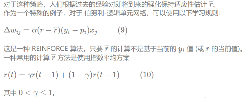
对于这种策略，人们根据过去的经验对即将到来的强化保持适应性估计 $\overline{r}$。
作为一个特殊的例子，对于 伯努利-逻辑单元网络，可以使用以下学习规则:
  ~  
$\Delta w_{ij}=\alpha (r-\overline{r})(y_i-p_i)x_j(9)$
  ~  
这是一种 REINFORCE 算法，只要 $\overline{r}$ 的计算不是基于当前的 $y_i$ 值 (或 $r$ 的当前值)。
一种常用的计算 $\overline{r}$ 方法是使用指数平均方案
  ~  
$\overline{r}(t)=\gamma r(t-1)+(1-\gamma )\overline{r}(t-1)(10)$
  ~  
其中 $0<\gamma \le 1$。
更复杂的策略也与 REINFORCE 框架相一致，包括将 当前输入模式 ${\mathbf{x}}^i$ 的函数 $\overline{r}$ 变成单元 。

虽然本文给出的分析结果没有提供对 REINFORCE 算法中各种 强化基线选择进行比较的依据，但一般认为，使用强化比较会使算法具有更好的性能。
我们将在下面以更长的篇幅讨论 REINFORCE 算法性能的问题。

5 回合式(Episodic) REINFORCE 算法

现在，我们考虑如何将 REINFORCE 类算法扩展到具有时间信用分配成分的某些学习问题，例如 网络包含环路或 环境提供未知的，可能是变化， 延迟的强化值。
特别是，假设一个网络 $N$ 是在逐个回合 的基础上训练的，其中每个回合 由 k 个时间步组成，在此期间，单元可以重新计算它们的输出，环境可以在每个时间步改变其对系统的非强化输入。
在每一个回合结束时，向网络传递一个单一的强化值 $r$。

该算法的推导基于“及时展开”映射的使用，该映射对于任意网络 $N$ 在固定时间段内运行的另一个网络 $N^{\ast }$ 没有循环，但表现出相应的行为。
每个时间步长复制 $N$ 一次，得到未展开的网络 $N^{\ast }$ 。
正式地，
$N$ 中 与时间有关的变量 $v$
$N^{\ast }$ 中时间索引的变量集 { v t } \{v^t\} {vt}， 其值不依赖于时间， 且对所有适当的 $t$， 有 $v(t)=v^t$
特别地， $N$ 中每个权重 $w_{ij}$ 产生 $N^{\ast }$ 中的一些权重 $w_{ij}^t$,
那些恰巧相等的所有值， 等于 $N$ 中的 $w_{ij}$ 的值,
因为它假定 $w_{ij}$ 在回合内是恒定的。

该问题可考虑的算法形式如下： 在每个回合结束时，每个参数 $w_{ij}$ 加上
  ~  
$\Delta w_{ij}={\alpha }_{ij}(r-b_{ij})\sum _{t=1}^k{e}_{ij}(t)(11)$
  ~  
其中所有符号与前面定义的相同，$e_{ij}(t)$ 表示 $w_{ij}$ 在特定时刻 $t$ 的特征合格性characteristic eligibility。
根据定义，$e_{ij}(t)=e_{ij}^t$
其中后者在无环网络 $N^{\ast }$ 中是有意义的。
例如，在同步更新的完全互连的伯努利-逻辑单元循环网络中，$e_{ij}(t)=(y_i(t)-p_i(t))x_j(t-1)$。
假设所有量都满足 REINFORCE 算法所需的相同条件，其中，特别是对于每个 $i$ 和 $j$ ，强化基线 $b_{ij}$ 独立于任何输出值 $y_i(t)$，速率因子 ${\alpha }_{ij}$ 最多依赖于 ${\mathbf{w}}^i$ 和 回合数。
将这种形式的任何算法(用于此类学习问题)称为回合式 REINFORCE 算法。

例如，如果网络由伯努利-逻辑单元组成，则回合式 REINFORCE 算法将根据该规则规定权重变化
  ~  
$\Delta w_{ij}={\alpha }_{ij}(r-b_{ij})\sum _{t=1}^k[y_i(t)-p_i(t)]x_j(t-1)$

以下结果在附录 A 中得到证明:

定理 2： 对于任何 回合式的 REINFORCE 算法， E { Δ W ∣ W } E\{\Delta {\bf W}|{\bf W}\} E{ΔW∣W} 和 ∇ w E { r ∣ W } \nabla _{\bf w}E\{r|{\bf W}\} ∇w​E{r∣W} 的内积是非负的。
更进一步，如果对所有 $i$ 和 $j$， 都有 ${\alpha }_{ij}$ > 0，那么只有当 ∇ w E { r ∣ W } = 0 \nabla _{\bf w}E\{r|{\bf W}\}=0 ∇w​E{r∣W}=0 时，这个内积才为 0。
同样，如果 ${\alpha }_{ij}=\alpha$ 独立于 $i$ 和 $j$，则 E { Δ W ∣ W } = α ∇ w E { r ∣ W } E\{\Delta {\bf W}|{\bf W}\} = \alpha \nabla _{\bf w}E\{r|{\bf W}\} E{ΔW∣W}=α∇w​E{r∣W}。

该算法值得注意的是，它有一个可行的在线实现，对网络中的每个参数 $w_{ij}$ 使用单个累加器。
该累加器的目的是形成合格和，其每一项仅取决于网络实时运行时的运行情况，而不取决于最终接收到的强化信号。

这种回合式学习任务的更一般的表述也是可能的，其中在回合的每个时间步都向网络传递强化，而不仅仅是在最后。
在这种情况下，合适的性能度量是 E { ∑ t − 1 k r ( t ) ∣ W } E\{\sum\limits_{t-1}^kr(t) |{\bf W}\} E{t−1∑k​r(t)∣W}。
为这种情况创建统计梯度跟踪算法的一种方法是简单地将 11 中的 $r$ 替换为 $\sum _{t-1}^{k}r(t)$，但有趣的是，当 $r$ 是因果关系时，因此它仅依赖于早期的网络输入和输出，可能有一种更好的方法来执行必要的信用分配。
粗略地说，我们的想法是将 $k$ 个时间步长的学习问题视为 $k$ 个不同但重叠的回合式学习问题，所有这些问题都从回合的开头开始。
我们省略了对这种方法细节的进一步讨论。

6 多参数分布 的 REINFORCE

例如，REINFORCE 框架的一个有趣应用是为单元开发学习算法，这些单元从多参数分布随机确定标量输出，而不是随机半线性单元使用的单参数分布。
这种单元以这种方式进行计算的一种方法是，它首先根据其权重和输入执行确定性计算，以获得控制随机数生成过程的所有参数的值，然后从近似的分布中随机提取其输出。
作为一个特殊的例子，正态分布有两个参数，均值 $\mu$ 和标准差 $\sigma$。
根据这种分布确定其输出 的单元将首先确定地计算 $\mu$ 和 $\sigma$ 的值，然后从平均值等于 μ 的值，标准差等于 $\sigma$ 的值的正态分布中得出其输出。

这种高斯单元的一个潜在有用的特征是，只要使用单独的权重(或者可能是输入)来确定这两个参数，其输出的均值和方差就可以单独控制。
有趣的是，对 $\sigma$ 的控制等同于对单元探索行为的控制。
一般来说，与使用单参数分布的随机单元不同，使用多参数分布的随机单元有可能控制其探索行为的程度，而不依赖于它们选择探索的位置。

在这里，我们注意到任何这样的单元的 REINFORCE 算法都很容易推导出来，使用高斯单元作为例子的特殊情况。
相比于承诺一个特定的方法来确定这样一个单元的输入和权重的输出的平均值和标准差，我们将简单地把这个单元，如果平均值和标准差本身作为单元的适应性参数。
这些参数对实际可适应参数和机组输入的任何更一般的函数依赖，只需应用链式法则。
Gullapalli(1990) 探索了计算这些参数的一种特殊方法，即在一组共同的输入行中使用单独的加权和(并使用某种不同的学习规则)。
为了简化表示法，我们只关注一个单元，且一如既往地忽略了通常的单元索引下标。

对于这样一个单元，可能输出的集合是实数的集合，决定任意一次试验输出 $y$ 的密度函数 $g$ 由下给定：
  ~  
$g(y,\mu ,\sigma )=\frac{1}{(2\pi {)}^{\frac{1}{2}}\sigma }{e}^{-\frac{(y-\mu {)}^2}{2{\sigma }^2}}$
  ~  
$\mu$ 的 characteristic eligibility 为：
  ~  
$\frac{\partial \ln g}{\partial \mu }=\frac{y-\mu }{{\sigma }^2}(12)$
  ~  
$\sigma$ 的 characteristic eligibility 为：
  ~  
$\frac{\partial \ln g}{\partial \sigma }=\frac{(y-\mu {)}^2-{\sigma }^2}{{\sigma }^3}$
  ~  
则这个单元的 REINFORCE 算法 具有以下形式：
  ~  
$\Delta \mu ={\alpha }_{\mu }(r-b_{\mu })\frac{y-\mu }{{\sigma }^2}(13)$
  ~  
且
  ~  
$\Delta \sigma ={\alpha }_{\sigma }(r-b_{\sigma })\frac{(y-\mu {)}^2-{\sigma }^2}{{\sigma }^3}(14)$
  ~  
其中 ${\alpha }_{\mu },b_{\mu },{\alpha }_{\sigma }$ 和 $b_{\sigma }$ 的选择是适当的。
通过以下设置得到了合理的算法：
  ~  
${\alpha }_{\mu }={\alpha }_{\sigma }=\alpha {\sigma }^2$
  ~  
其中 $\alpha$ 为适当小的正常数${}^2$ ，令 $b_{\mu }=b_{\sigma }$，根据强化比较方案确定。

脚注 2：严格来说，除非正态分布的尾部被截断 (这在实践中是必然的情况)，否则该算法 无论如何 选 $\alpha$ 都无法保证 $\sigma$ 不会变为负值。
另一种方法是令 $\lambda =\ln \sigma$ 作为自适应参数，而不是 $\sigma$，这样可以保证算法保持 $\sigma$ 为正。

有趣的是，方程 (12) 给出了正态分布参数 $\mu$ 的特征合格性characteristic eligibility ，而方程 (5) 给出了伯努利分布参数 $p$ 的特征合格性characteristic eligibility 。
由于 $p$ 是相应伯努利随机变量的均值，$p(1-p)$ 是相应伯努利随机变量的方差，因此两个方程具有相同的形式。
事实上，对于更广泛的分布，平均参数的特征合格性characteristic eligibility 具有这种形式，如下结果所示:

命题 1 假设概率质量或密度函数 $g$ 有这样的形式：
$g(y,\mu ,{\theta }_2,\cdots ,{\theta }_k)=\exp [Q(\mu ,{\theta }_2,\cdots ,{\theta }_k)]y+D(\mu ,{\theta }_2,\cdots ,{\theta }_k)+S(y)$
$Q,D,S$ 为函数， $\mu ,{\theta }_2,\cdots ,{\theta }_k$ 为参数。 $\mu$ 是分布的均值。
$\frac{\partial \ln g}{\partial \mu }=\frac{y-\mu }{{\sigma }^2}$
其中 ${\sigma }^2$ 是分布的方差

具有这种形式的质量或密度函数表示指数族分布的特殊情况(Rohatgi, 1976)。
我们很容易发现，许多我们熟悉的分布，如泊松分布、指数分布、伯努利分布和正态分布，都是这种形式。
这个命题的证明在附录 B 中给出。

7 与反向传播的兼容性

It is useful to note that REINFORCE, like most other reinforcement learning algorithms for networks of stochastic units, works essentially by measuring the correlation between variations in local behavior and the resulting variations in global performance, as given by the reinforcement signal.
值得注意的是，与大多数其他用于随机单元网络的强化学习算法一样，REINFORCE 的工作原理基本上是通过测量局部行为变化与由此产生的全局性能变化之间的相关性来实现的，正如强化信号所给出的那样。
When such algorithms are used, all information about the effect of connectivity between units is ignored; each unit in the network tries to determine the effect of changes of its output on changes in reinforcement independently of its effect on even those units to which it is directly connected.
当使用这种算法时，所有关于单元之间连通性影响的信息都被忽略;
网络中的每个单元都试图确定其输出变化 对强化变化的影响，而不依赖于其对直接连接的单元的影响。
In contrast, the backpropagation algorithm works by making use of the fact that entire chains of effects are predictable from knowledge of the effects of individual units on each other.
相反，反向传播算法的工作原理利用了这样一个事实，即整个影响链是可以通过了解单个单元对彼此的影响来预测的。
While the backpropagation algorithm is appropriate only for supervised learning in networks of deterministic units, it makes sense to also use the term backpropagation for the single component of this algorithm that determines relevant partial derivatives by means of the backward pass.
反向传播算法仅适用于确定性单元网络中的监督学习，但也可以将术语反向传播用于该算法的单个组件，该算法通过反向传递确定相关的偏导数。
(In this sense it is simply a computational implementation of the chain rule.)
With this meaning of the term we can then consider how backpropagation might be integrated into the statistical gradient-following reinforcement learning algorithms investigated here, thereby giving rise to algorithms that can take advantage of relevant knowledge of network connectivity where appropriate.
(从这个意义上说，它只是链式法则的计算实现。)
有了这个术语的含义，我们就可以考虑如何将反向传播集成到这里研究的统计梯度跟随强化学习算法中，从而产生可以在适当的地方利用网络连接相关知识的算法。
Here we examine two ways that backpropagation can be used.
这里我们研究可以使用的反向传播的两种方法。

7.1 使用 确定性单元 的 网络

Consider a feedforward network having stochastic output units and deterministic hidden units.
考虑一个具有随机输出单元 和 确定隐藏单元的前馈网络。
Use of such a network as a reinforcement learning system makes sense because having randomness limited to the output units still allows the necessary exploration to take place.
使用这种网络作为强化学习系统是有意义的，因为将随机性限制在输出单元中仍然允许进行必要的探索。

设 $\mathbf{x}$ 表示网络输入向量，$\mathbf{y}$ 表示网络输出向量。
我们可以定义 g ( ξ , W , x ) = Pr { y = ξ ∣ W , x } g(\xi,{\bf W},{\bf x}) = \text{Pr} \{y=\xi| {\bf W},{\bf x}\} g(ξ,W,x)=Pr{y=ξ∣W,x} 为描述整个网络的输入-输出行为的总体概率质量函数。
除了网络的输出通常是矢量值而不是标量值这一事实之外，当采用全局而不是局部视角时，用于推导 REINFORCE 算法的形式 和参数几乎没有变化。
特别地，将证明定理 1 的论证简单推广到向量值输出的情况，表明对于网络中的任意权重 $w_{ij}$， $(r-b_{ij})\frac{\partial \ln g}{\partial w_{ij}}$ 表示 ∂ E { r ∣ W } ∂ w i j \frac{\partial E\{r|{\bf W}\}}{\partial w_{ij}} ∂wij​∂E{r∣W}​ 的无偏估计。

设 $O$ 表示输出单元的索引集。
因为所有的随机性都存在于输出单元中，并且因为随机性在这些单元之间是独立的，我们有
  ~  
Pr { y = ξ ∣ W , x } = ∏ k ∈ O Pr { y k = ξ k ∣ W , x } = ∏ k ∈ O Pr { y k = ξ k ∣ w k , x k } \begin{aligned}\text{Pr}\{{\bf y}=\xi|{\bf W}, {\bf x}\} &=\prod\limits_{k\in O}\text{Pr}\{y_k=\xi_k|{\bf W}, {\bf x}\}\\ &=\prod\limits_{k\in O}\text{Pr}\{y_k=\xi_k|{\bf w}^k, {\bf x}^k\}\end{aligned} Pr{y=ξ∣W,x}​=k∈O∏​Pr{yk​=ξk​∣W,x}=k∈O∏​Pr{yk​=ξk​∣wk,xk}​
  ~  
其中，对于每个 $k$, ${\mathbf{x}}^k$ 是出现在第 $k$ 个单元的输入处的模式，这是将模式 $\mathbf{x}$ 呈现给网络的结果。
注意，每个 ${\mathbf{x}}^k$ 都确定地依赖于 $\mathbf{x}$ 。

↓ 在这里， ln 将 连乘运算 转成 求和运算

因此
$\ln g(\xi ,\mathbf{W},\mathbf{x})=\ln \prod _{k\in O}{g}_k({\xi }_k,{\mathbf{w}}^k,{\mathbf{x}}^k)=\sum _{k\in O}\ln g_k({\xi }_k,{\mathbf{w}}^k,{\mathbf{x}}^k)$
  ~  
$\frac{\partial \ln g}{\partial w_{ij}}(\xi ,\mathbf{W},\mathbf{x})=\sum _{k\in O}\frac{\partial \ln g_k}{\partial w_{ij}}({\xi }_k,{\mathbf{w}}^k,{\mathbf{x}}^k)$

显然，这个和可以通过反向传播计算出来。
例如，当输出单元为伯努利半线性单元时，我们可以使用参数 $p_k$ 作为中间变量，并写出任意权重 $w_{ij}$ 的特征合格性 characteristic eligibility:
  ~  
$\frac{\partial \ln g}{\partial w_{ij}}=\sum _{k\in O}\frac{\partial \ln g_k}{\partial p_k}\frac{\partial p_k}{\partial w_{ij}}$
  ~  
这是通过“注入”injecting 来有效计算的
  ~  
$\frac{\partial \ln g_k}{\partial p_k}=\frac{y_k-p_k}{p_k(1-p_k)}$
  ~  
就在 第 $k$ 个单元的压缩函数之后，
对于每个 $k$，然后执行标准的向后传递。
注意，如果 $w_{ij}$ 是附加在输出单元上的权重，则此反向传播计算只会产生前面导出的结果 (6)。
对于这个结果，我们本质上通过由“压碎机”“squasher” 和“夏季” “summer.” 组成的子单元反向传播伯努利参数 $p_i$ 的特征合格性characteristic eligibility 。

While we have restricted attention here to networks having stochastic output units only,it is not hard to see that such a result can be further generalized to any network containing an arbitrary mixture of stochastic and deterministic units.
我们在这里限制了对只有随机输出单元的网络的关注，但不难看出，这样的结果可以进一步推广到任何包含随机和确定性单元任意混合的网络。
The overall algorithm in this case consists of the use of the correlation-style REINFORCE computation at each stochastic unit, whether an output unit or not, with backpropagation used to compute (or, more precisely, estimate) all other relevant partial derivatives.
在这种情况下，整个算法包括在每个随机单元(无论是否为输出单元)上使用相关风格的 REINFORCE 计算，并使用反向传播来计算(或者更准确地说，估计)所有其他相关的偏导数。

Furthermore, it is not difficult to prove an even more general compatibility between computation of unbiased estimates, not necessarily based on REINFORCE, and backpropagation through deterministic functions.
此外，在无偏估计的计算(不一定基于 REINFORCE ) 和 通过确定性函数的反向传播之间证明一种更普遍的兼容性并不困难。
The result is, essentially, that when one set of variables depends deterministically on a second set of variables, backpropagating unbiased estimates of partial derivatives with respect to the first set of variables gives rise to unbiased estimates of partial derivatives with respect to the second set of variables.
结果是，本质上，当一组变量确定地依赖于另一组变量时，对第一组变量的偏导数的反向传播无偏估计会产生对第二组变量的偏导数的无偏估计。
It is intuitively reasonable that this should be true, but we omit the rigorous mathematical details here since we make no use of the result.
直觉上，这应该是合理的，但我们省略了严格的数学细节，因为我们没有使用这个结果。

7.2 通过随机数生成器 进行 反向传播

刚才描述的算法形式利用了网络的确定性部分内的反向传播，但每当需要在随机数生成器的输入端获得偏导数信息时，它仍然需要相关风格correlation-style 的计算。
相反，假设有可能以某种方式“通过随机数生成器反向传播”。
为了了解这可能意味着什么，考虑一个随机半线性单元，并假设有一个函数 $J$ 对输出 $y_i$ 具有某种确定性依赖。
这种情况的一个例子是，当单元是输出单元时， J = E { r ∣ W } J = E\{r|{\bf W}\} J=E{r∣W}，强化取决于网络输出是否正确。
粗略地说，我们想要的是能够根据 $\frac{\partial J}{\partial y_i}$ 的知识 计算 $\frac{\partial J}{\partial p_i}$。
然而，由于随机性，我们不能期望这些数量之间存在确定的关系。
一个更合理的要求属性是 ∂ E { J ∣ p i } ∂ p i \frac{\partial E\{ J|p_i\}}{\partial p_i} ∂pi​∂E{J∣pi​}​ 由 E { ∂ J ∂ y i ∣ p i } E\{\frac{\partial J}{\partial y_i}|p_i\} E{∂yi​∂J​∣pi​} 确定。

不幸的是，即使这个性质在一般情况下也不成立。
例如，在伯努利单元中，很容易检查当 $J$ 是 $y_i$ 的非线性函数时，这两个量之间不需要有特殊的关系。
但是，如果随机数生成器的输出可以写成其参数的可微函数，刚才描述的通过确定性计算进行反向传播的方法是可行的。

作为一个例子，考虑一个正态随机数生成器，在高斯单元中使用。
它的输出 $y$ 是根据参数 $\mu$ 和 $\sigma$ 随机生成的，我们可以写成
  ~  
$y=\mu +\sigma z$
  ~  
其中 $z$ 是标准正态偏差。则
  ~  
$\frac{\partial y}{\partial \mu }=1$
  ~  
$\frac{\partial y}{\partial \sigma }=z=\frac{y-\mu }{\sigma }$
  ~  
因此，例如，可以将通过高斯隐藏单元的反向传播 与 输出单元中的 REINFORCE 相结合。
在这种情况下，这种单元中 $\mu$ 的characteristic eligibility 被设置为等于为输出值 $y$ 计算的特征资格characteristic eligibility ，而参数 $\sigma$ 的特征资格characteristic eligibility 通过将 $y$ 的特征资格characteristic eligibility 乘以 $\frac{y-\mu }{\sigma }$ 获得。
值得注意的是，这些特定的结果绝不取决于 $\mu$ 是平均值，$\sigma$ 是标准差;
当 $\mu$ 表示分布的转换参数和 $\sigma$ 表示分布的缩放参数时，同样的结果也适用。
更一般地说，只要输出可以表示为参数和一些辅助随机变量的函数，只要对参数的依赖是可微的，显然可以使用相同的技术。

Note that the argument given here is based on the results obtained above for the use of backpropagation when computing the characteristic eligibility in a REINFORCE algorithm, so the conclusion is necessarily limited to this particular use of backpropagation here.
注意，这里给出的论证是基于上面在计算 REINFORCE 算法中的特征合格性characteristic eligibility 时使用反向传播获得的结果，因此结论必然限于这里的反向传播的这种特殊使用。
Nevertheless, because it is also true that backpropagation preserves the unbiasedness of gradient estimates in general, this form of argument can be applied to yield statistical gradient-following algorithms that make use of backpropagation in a variety of other situations where a network of continuous-valued stochastic units is used.
然而，由于反向传播在一般情况下保持梯度估计的无偏性也是正确的，因此这种形式的论证可以应用于产生统计梯度跟踪算法，这些算法在使用 连续值随机单元网络 的各种其他情况下使用反向传播。
One such application is to supervised training of such networks.
其中一个应用就是对这种网络进行监督训练。

8 算法性能 和 其它问题

8.1 收敛性能

A major limitation of the analysis performed here is that it does not immediately lead to prediction of the asymptotic properties of REINFORCE algorithms.
这里进行的分析的一个主要限制是，它不能立即获得对 REINFORCE 算法的渐近性质的预测。
If such an algorithm does converge, one might expect it to converge to a local maximum, but there need be no such convergence.
如果这样的算法确实收敛，人们可能期望它收敛到局部最大值，但不需要这样的收敛。
While there is a clear need for an analytical characterization of the asymptotic behavior of REINFORCE algorithms, such results are not yet available, leaving simulation studies as our primary source of understanding of the behavior of these algorithms.
显然需要对 REINFORCE 算法的渐近行为进行分析表征，但目前还没有这样的结果，因此模拟研究是我们理解这些算法行为的主要来源。
Here we give an overview of some relevant simulation results, some of which have been reported in the literature and some of which are currently only preliminary.
在这里，我们概述了一些相关的模拟结果，其中一些已经在文献中报道，其中一些目前只是初步的。

Sutton (1984) studied the performance of a number of algorithms using single-Bernoulliunit “networks” facing both nonassociative and associative immediate-reinforcement tasks.
Among the algorithms investigated were LR-I and one based on equations (9) and (10), which is just REINFORCE using reinforcement comparison.
所研究的算法中有基于式 (9) 和式 (10) 的 $L_{R-I}$，只有 REINFORCE 使用强化比较reinforcement comparison。

In these studies, REINFORCE with reinforcement comparison was found to outperform all other algorithms investigated.
在这些研究中，发现 带强化比较reinforcement comparison 的 REINFORCE 优于所有其他研究算法。

Williams and Peng (1991) have also investigated a number of variants of REINFORCE in nonassociative function-optimization tasks, using networks of Bernoulli units.
Williams 和 Peng(1991) 也使用伯努利单元网络 研究了非联想函数优化任务中 REINFORCE 的多种变体。
These might expect of any gradient-following algorithm.
这可能是任何梯度跟随算法的结果。
Some of the variants examined incorporated modifications designed to help defeat this often undesirable behavior.
一些被检查的变体包含了旨在帮助克服这种通常不受欢迎的行为的修改。
One particularly interesting variant incorporated an entropy term in the reinforcement signal and helped enable certain network architectures to perform especially well on tasks where a certain amount of hierarchical organization during the search was desirable.
一个特别有趣的变体在强化信号中加入了熵项，并帮助某些网络架构在搜索过程中需要一定数量的分层组织的任务中表现得特别好。

Other preliminary studies have been carried out using networks of Bernoulli units and using single Gaussian units.
其他的初步研究已经使用伯努利单元网络 和 使用单个高斯单元进行。
The Gaussian unit studies are described below.
下面描述高斯单元的研究。
The network studies involved multilayer or recurrent networks facing supervised learning tasks but receiving only reinforcement feedback.
网络研究涉及多层或循环网络面向监督学习任务，但只接受强化反馈。
In the case of the recurrent networks, the objective was to learn a trajectory and episodic REINFORCE was used.
在循环网络的情况下，目标是学习一个轨迹，并使用回合式 REINFORCE。
One of the more noteworthy results of these studies was that it often required careful selection of the reinforcement function to obtain solutions using REINFORCE.
这些研究的一个更值得注意的结果是，通常需要仔细选择强化函数来获得使用 REINFORCE 的解决方案。
This is not surprising since it turns out that some of the more obvious reinforcement functions one might select for such problems tend to have severe false maxima.
这并不奇怪，因为事实证明，人们可能为这类问题选择的一些更明显的强化函数往往具有严重的假最大值。
In contrast, $A_{R-P}$ generally succeeds at finding solutions even when these simpler reinforcement functions are used.
相比之下，即使使用了这些更简单的强化函数，$A_{R-P}$ 通常也能成功地找到解决方案。
Like $A_{R-P}$ , REINFORCE is generally very slow even when it succeeds. Episodic REINFORCE has been found to be especially slow, but this, too, is not surprising since it performs temporal credit-assignment by essentially spreading credit or blame uniformly over all past times.
与 $A_{R-P}$ 一样，REINFORCE 通常也非常缓慢，即使它成功了。
回合式 REINFORCE 被发现特别缓慢，但也这不足为奇，因为它通过在所有过去的时间里统一地传播功劳credit 或指责blame 来执行时序的 credit-assignment。

One REINFORCE algorithm whose asymptotic behavior is reasonably well understood analytically is 2-action $L_{R-I}$, and simulation experience obtained to date with a number of other REINFORCE algorithms suggests that their range of possible limiting behaviors may, in fact, be similar.
有一种 REINFORCE 算法，其渐近行为可以很好地解析理解为 2-action $L_{R-I}$，并且迄今为止与许多其他 REINFORCE 算法获得的模拟经验表明，它们可能的极限行为范围实际上可能是相似的。
The $L_{R-I}$ algorithm is known to converge to a single deterministic choice of action with probability 1.
已知 $L_{R-I}$ 算法收敛于概率为 1 的单个确定性行为选择。
What is noteworthy about this convergence is that,in spite of the fact that the expected motion is always in the direction of the best action,as follows from Theorem 1, there is always a nonzero probability of its converging to an inferior choice of action.
关于这种收敛，值得注意的是，尽管预期运动总是在最佳行动的方向上，根据定理 1，它总是有一个非零概率收敛到一个较差的行动选择。
A simpler example that exhibits the same kind of behavior is a biased random walk on the integers with absorbing barriers.
表现出相同行为的一个更简单的例子是对具有吸收障碍的整数的有偏随机漫步。
Even though the motion is biased in a particular direction, there is always a nonzero probability of being absorbed at the other barrier.
即使运动偏向于一个特定的方向，被另一个势垒吸收的概率也总是非零的。

In general, a reasonable conjecture consistent with what is known analytically about simple REINFORCE algorithms like $L_{R-I}$ and what has been found in simulations of more sophisticated REINFORCE algorithms is the following: Depending on the choice of reinforcement baseline used, any such algorithm is more or less likely to converge to a local maximum of the expected reinforcement function, with some nonzero (but typically comfortably small) probability of convergence to other points that lead to zero variance in network behavior.
总的来说，一个合理的推测符合我们对简单的 REINFORCE 算法(如 $L_{R-I}$ )的解析性了解，以及在更复杂的 REINFORCE 算法的模拟中发现的结果：
根据所使用的增强基线的选择，任何这样的算法或多或少都有可能收敛到预期强化函数的局部最大值，并且收敛到导致网络行为零方差的其他点的概率为非零(但通常非常小)。
For further discussion of the role of the reinforcement baseline, see below.
关于强化基线作用的进一步讨论，见下文。

8.2 高斯单元 搜索行为

对于上述提及的高斯单元研究，所考虑的问题是非关联的，涉及单个实变量 $y$ 的函数的优化，且自适应参数取为 $\mu$ 和 $\sigma$。
从方程 13 和 14 可以清楚地看出，该单元的强化比较reinforcement comparison 版本的 REINFORCE 表现如下：
如果采样值 $y$ 导致比最近获得的函数值更高，则 $\mu$ 向 $y$ 移动;
类似地，$\mu$ 从给出较低函数值的点移开。
更有趣的是 $\sigma$ 是如何适应的。
如果采样点 $y$ 产生的函数值比最近获得的函数值高，则当 $|y-\mu |<\sigma$ 时，$\sigma$ 将减小，当 $|y-\mu |>\sigma$ 时，$\sigma$ 将增大。
$\sigma$ 所做的变化 对应于 使 $y$ 更有可能再次出现所需的变化。
如果采样点导致一个较低的值，则有相反方向的相应行为。
就搜索而言，如果在 均值$\mu$ 附近找到一个较好的点，或者在远离均值的地方找到一个较差的点，这相当于将搜索范围缩小到 $\mu$ 附近。
如果在 均值附近找到一个较差的点，或者在远离均值的地方找到一个较好的点，这相当于扩大 $\mu$ 附近的搜索范围。
由于采样点 $y$ 在平均值的一个标准差内的可能性大约是平均值的两倍，因此，每当 $\mu$ 位于局部山丘的顶部(相对于 $\sigma$ 有足够的宽度)时，$\sigma$ 就会缩小以允许收敛到局部最大值。
然而，如果局部最大值在顶部非常平坦，$\sigma$ 也会减小到 采样更差值变得极不可能 的点，然后停止变化。
使用确定性和噪声强化的仿真研究证实了这一行为。
他们还证明，如果 $r$ 总是非负的，并且不使用强化比较 reinforcement comparison (即，b = 0)，REINFORCE 可能导致 $\sigma$ 在 $\mu$ 移动到任何山顶之前收敛到 0。这可以看作是前面描述的 $L_{R-I}$ 潜在收敛到次优性能的推广。

将这种单元的 REINFORCE 与 Gullapalli(1990) 提出的用于适应 $\mu$ 和 $\sigma$ 的替代算法进行比较是很有趣的。
在这种方法中，$\mu$ 的适应方式与 REINFORCE 中的基本相同，而 $\sigma$ 的适应方式则完全不同。
假设强化值 $r$ 介于 0 和 1 之间，则取 $\sigma$ 与 $1-r$ 成正比。
如果认为 $\sigma$ 是控制正在执行的搜索规模的参数，并且函数的最佳值是未知的，则此策略是有意义的。
在这些情况下，当知道实现了不满意的性能时，扩大这个范围是合理的，以便对搜索空间采取粗粒度视图，并确定一个广泛的区域，在该区域中有合理的机会找到最优。

Also relevant here is the work of Schmidhuber and Huber (1990), who have reported successful results using networks having Gaussian output units in control tasks involving backpropagating through a model (Jordan & Rumelhart, 1990).
Schmidhuber 和 Huber(1990) 的工作也与此相关，他们报告了使用具有高斯输出单元的网络在控制任务中通过模型进行反向传播的成功结果(Jordan & Rumelhart, 1990)。
In this work, backpropagation through random number generators was used to allow learning of a model and learning of performance to proceed simultaneously rather than in separate phases.
在这项工作中，通过随机数生成器的反向传播 被用于让模型学习和性能学习同时进行，而不是在单独的阶段进行。

8.3 强化基线 的选择

这里给出的分析的一个重要限制是，它没有提供在 REINFORCE 算法中各种 强化基线选择的依据。
虽然定理 1 同样适用于任何此类选择，但对此类算法的广泛实证调查得出了不可避免的结论，即使用自适应强化基线 结合 强化比较 策略可以大大提高收敛速度，并且在某些情况下，也可以导致定性行为的巨大差异。
上面描述的高斯单元研究给出了一个例子。
一个更简单的例子是一个单一的伯努利半线性单元，只有一个偏置权重和输入，其输出 $y$ 确定性地影响强化 $r$。
如果 $r$ 总是正的，很容易看出，当 $b=0$ 时，得到一种有偏的随机漫步行为，导致收敛到次输出值的概率非零。
相比之下，强化比较 版本将导致 $b$ 的值介于 $r$ 的两个可能值之间，从而导致运动总是朝着更好的输出值。

然而，对于位于 $r$ 的两个可能值之间的 $b$ 的任何选择，后一种行为都会发生，因此必须应用额外的考虑来区分各种可能的自适应强化基线方案。
Williams(1986) 简要地考虑了一种可能性，Dayan(1990) 最近对其进行了更全面的研究，即选择一个使单独的权重随时间变化的方差最小化的强化基线。
结果证明，这不是通常的强化比较方法中的平均强化，而是另一个更难有效估计的量。
Dayan 的模拟结果似乎表明，与使用均值强化相比，使用这样的强化基线对于收敛速度略有改善，但更令人信服的优势仍有待证明。

8.4 eligibility 的形式选择

REINFORCE, with or without reinforcement comparison, prescribes weight changes proportional to the product of a reinforcement factor that depends only on the current and past reinforcement values and another factor we have called the characteristic eligibility.
无论有无 强化比较reinforcement comparison，REINFORCE 都规定了权重变化与 仅取决于当前和过去强化值的强化系数 和 我们称之为特征合格性characteristic eligibility 的另一个因素的乘积 成正比。
A straightforward way to obtain a number of variants of REINFORCE is to vary the form of either of these factors.
获得 REINFORCE 的一些变体的一个直接方法是改变这些因素中的任何一个的形式。
Indeed, the simulation study performed by Sutton (1984) involved a variety of algorithms obtained by systematically varying both of these factors.
事实上，Sutton(1984) 进行的模拟研究涉及通过系统地改变这两个因素而获得的各种算法。
One particularly interesting variant having this form but not included in that earlier study has since been examined by several investigators (Rich Sutton, personal communication, 1986; Phil Madsen, personal communication, 1987; Williams & Peng, 1991) and found promising.
一个特别有趣的变体有这种形式，但没有包括在早期的研究中，后来被几位研究者研究过((Rich Sutton, personal communication, 1986; Phil Madsen, personal communication, 1987; Williams & Peng, 1991) )，发现很有前景。
These studies have been conducted only for nonassociative tasks, so this is the form of the algorithm we describe here.
这些研究只针对非联想任务进行，所以这就是我们在这里描述的算法的形式。
(Furthermore, because a principled basis for deriving algorithms of this particular form has not yet been developed, it is somewhat unclear exactly how it should be extended to the associative case.)
(此外，由于导出这种特殊形式的算法的原则基础尚未开发，因此如何将其扩展到关联情况有些不清楚。)

我们特别考虑 伯努利-逻辑单元 只有偏置权重 $w$ 的情况。
由于偏置输入为 1，REINFORCE 的标准 强化比较 版本规定了这种形式的权重增量：
  ~  
$\Delta w=\alpha (r-\bar{r})(y-p)$
  ~  
其中 $\bar{r}$ 根据指数平均方案 计算
  ~  
$\bar{r}(t)=\gamma r(t-1)+(1-\gamma )\bar{r}(t-1)$
  ~  
其中 $0<\gamma <1$。该规则给出了一种替代算法
  ~  
$\Delta w=\alpha (r-\bar{r})(y-\bar{y})$
  ~  
其中 $\bar{y}$ 根据下式进行更新：
  ~  
$\bar{y}(t)=\gamma y(t-1)+(1-\gamma )\bar{y}(t-1)$
  ~  
使用与更新 $\bar{r}$ 相同的 $\gamma$ 。
这种特殊的算法通常比相应的 REINFORCE 算法收敛得更快，更可靠。

很明显，这两种算法有很强的相似性。
变体是通过简单地用 $\bar{y}$ 替换 $p$ 来获得的，其中每一个都可以被视为对输出 $y$ 的合理先验估计。
此外，在许多其他情况下，相应的策略可以用于生成 REINFORCE 的变体。
例如，如果单元中的随机性使用命题 1 适用的任何分布，那么用于调整其平均值参数 $\mu$ 的 REINFORCE 算法将涉及因子 $y-\mu$，我们可以简单地替换成 $y-\bar{y}$。
这种适应高斯单元均值的算法已经经过测试，并且表现得非常好。

虽然可以给出一些论证 (Rich Sutton, personal communication, 1988)，表明在这种算法中使用 $y-\bar{y}$ 的潜在优势，但尚未进行更完整的分析。
有趣的是，使用这种算法的一个可能的分析理由可以在下面讨论的考虑中找到。

8.5 其它局部梯度估计的使用

There are several senses in which it makes sense to call REINFORCE algorithms simple, as implied by the title of this paper.
就像本文的标题所暗示的那样，在几个意义上说 REINFORCE 算法简单是合理的。
First, as is clear from examples given here, the algorithms themselves often have a very simple form.
首先，从这里给出的例子可以清楚地看出，算法本身通常具有非常简单的形式。
Also, they are simple to derive for essentially any form of random unit computation.
此外，对于任何形式的随机单位计算，它们都很容易推导出来。
But perhaps most significant of all is the fact that, in the sense given by Theorems 1 and 2, they climb an appropriate gradient without explicitly computing any estimate of this gradient or even storing information from which such an estimate could be directly computed.
但也许最重要的是，在定理 1 和定理 2 给出的意义上，它们爬上一个适当的梯度，而不显式地计算这个梯度的任何估计，甚至不存储可以直接计算这种估计的信息。
Clearly, there are alternative ways to estimate such gradients and it would be useful to understand how various such techniques can be integrated effectively.
显然，有其他方法来估计这种梯度，了解如何有效地集成各种这样的技术将是有用的。

---

↓ 【model-based】

To help distinguish among a variety of alternative approaches, we first define some terminology.
为了帮助区分各种可选方法，我们首先定义一些术语。
Barto, Sutton, and Watkins (1990), have introduced the term model-based to describe what essentially correspond to indirect algorithms in the adaptive control field (Goodwin & Sin, 1984).
Barto, Sutton 和 Watkins(1990) 引入了术语“基于模型”来描述自适应控制领域中本质上对应于间接算法的内容(Goodwin & Sin, 1984)。
These algorithms explicitly estimate relevant parameters underlying the system to be controlled and then use this learned model of the system to compute the control actions.
这些算法明确地估计待控制系统的相关参数，然后使用该系统的学习模型来计算控制动作。
The corresponding notion for an immediate-reinforcement learning system would be one that attempts to learn an explicit model of the reinforcement as a function of learning system input and output, and use this model to guide its parameter adjustments.
对于立即强化学习系统，相应的概念是尝试学习强化的显式模型，作为学习系统输入和输出的函数，并使用该模型来指导其参数调整。
If these parameter adjustments are to be made along the gradient of expected reinforcement, as in REINFORCE, then this model must actually yield estimates of this gradient.
如果这些参数调整是沿着预期强化的梯度进行的，如在 REINFORCE 中，那么这个模型必须 实际上产生这个梯度的估计。
Such an algorithm, using backpropagation through a model, has been proposed and studied by Munro (1987).
Munro(1987) 提出并研究了这种通过模型进行反向传播的算法。

This form of model-based approach uses a global model of the reinforcement function and its derivatives, but a more local model-based approach is also possible.
这种形式的基于模型的方法使用强化函数及其衍生物的全局模型，但更局部的基于模型的方法也是可能的。
This would involve attempting to estimate, at each unit, the expected value of reinforcement as a function of input and output of that unit, or, if a gradient algorithm like REINFORCE is desired, the derivatives of this expected reinforcement.
这将涉及尝试估计，在每个单元，强化的期望值作为该单元的输入和输出的函数，或者，如果需要像 REINFORCE 这样的梯度算法，则为这个强化期望值的导数。
An algorithm studied by Thathatchar and Sastry (1985) for stochastic learning automata keeps track of the average reinforcement received for each action and is thus of this general form.
Thathatchar 和 Sastry(1985) 研究的随机学习自动机的算法 跟踪每个动作接收到的平均强化，因此具有这种一般形式。
Q-learning (Watkins, 1989) can also be viewed as involving the learning of local (meaning, in this case, per-state) models for the cumulative reinforcement.
Q-learning (Watkins, 1989) 也可以被视为涉及累积强化的局部(在这种情况下是指每个状态)模型的学习。

REINFORCE fails to be model-based even in this local sense, but it may be worthwhile to consider algorithms that do attempt to generate more explicit gradient estimates if their use can lead to algorithms having clearly identifiable strengths.
即使在这种局部意义上，REINFORCE 也不是基于模型的，但是如果使用它们可以让算法具有明确可识别的优势，那么考虑尝试生成更显式梯度估计的算法可能是值得的。
One interesting possibility that applies at least in the nonassociative case is to perform, at each unit, a linear regression of the reinforcement signal on the output of the unit.
至少在非关联情况下适用的一个有趣的可能性是，在每个单元上对单元的输出执行强化信号的线性回归。
It is suspected that algorithms using the $y-\bar{y}$ form of eligibility described above may be related to such an approach but this has not been fully analyzed yet.
怀疑使用上述 $y-\bar{y}$ 形式的资格eligibility 的算法可能与这种方法有关，但尚未对此进行充分分析。

9 结论

The analyses presented here, together with a variety of simulation experiments performed by this author and others, suggest that REINFORCE algorithms are useful in their own right and, perhaps more importantly, may serve as a sound basis for developing other more effective reinforcement learning algorithms. 【总体概括】
本文的分析以及作者和其他人进行的各种模拟实验表明，REINFORCE 算法本身是有用的，也许更重要的是，可以作为开发其他更有效的强化学习算法的坚实基础。
One major advantage of the REINFORCE approach is that it represents a prescription for devising statistical gradient-following algorithms for reinforcement-learning networks of units that compute their random output in essentially any arbitrary fashion. 【优点 1】
REINFORCE 方法的一个主要优点是，它代表了为强化学习网络设计统计梯度跟随算法的处方，这些网络的单元基本上可以任意方式计算其随机输出。
Also, because it is a gradient-based approach, it integrates well with other gradient computation techniques such as backpropagation.
此外，由于它是一种基于梯度的方法，它可以很好地与其他梯度计算技术(如反向传播)集成。【优点 2】
The main disadvantages are the lack of a general convergence theory applicable to this class of algorithms and, as with all gradient algorithms, an apparent susceptibility to convergence to false optima. 【缺点】
其主要缺点是缺乏适用于这类算法的一般收敛理论，并且与所有梯度算法一样，明显容易收敛到假最优。

致谢

I have benefitted immeasurably from numerous discussions with Rich Sutton and Andy Barto on various aspects of the material presented herein. Preparation of this paper was supported by the National Science Foundation under grant IRI-8921275.
我与 Rich Sutton 和 Andy Barto 就本文所介绍的材料的各个方面进行了无数次讨论，从中受益匪浅。
本文由美国国家科学基金资助，项目编号为 IRI-8921275。

剩余部分： 【论文_1992】 REINFORCE » P2 附录