


👨🎓个人主页:研学社的博客
💥💥💞💞欢迎来到本博客❤️❤️💥💥
🏆博主优势:🌞🌞🌞博客内容尽量做到思维缜密,逻辑清晰,为了方便读者。
⛳️座右铭:行百里者,半于九十。
📋📋📋本文目录如下:🎁🎁🎁
目录

💥1 概述
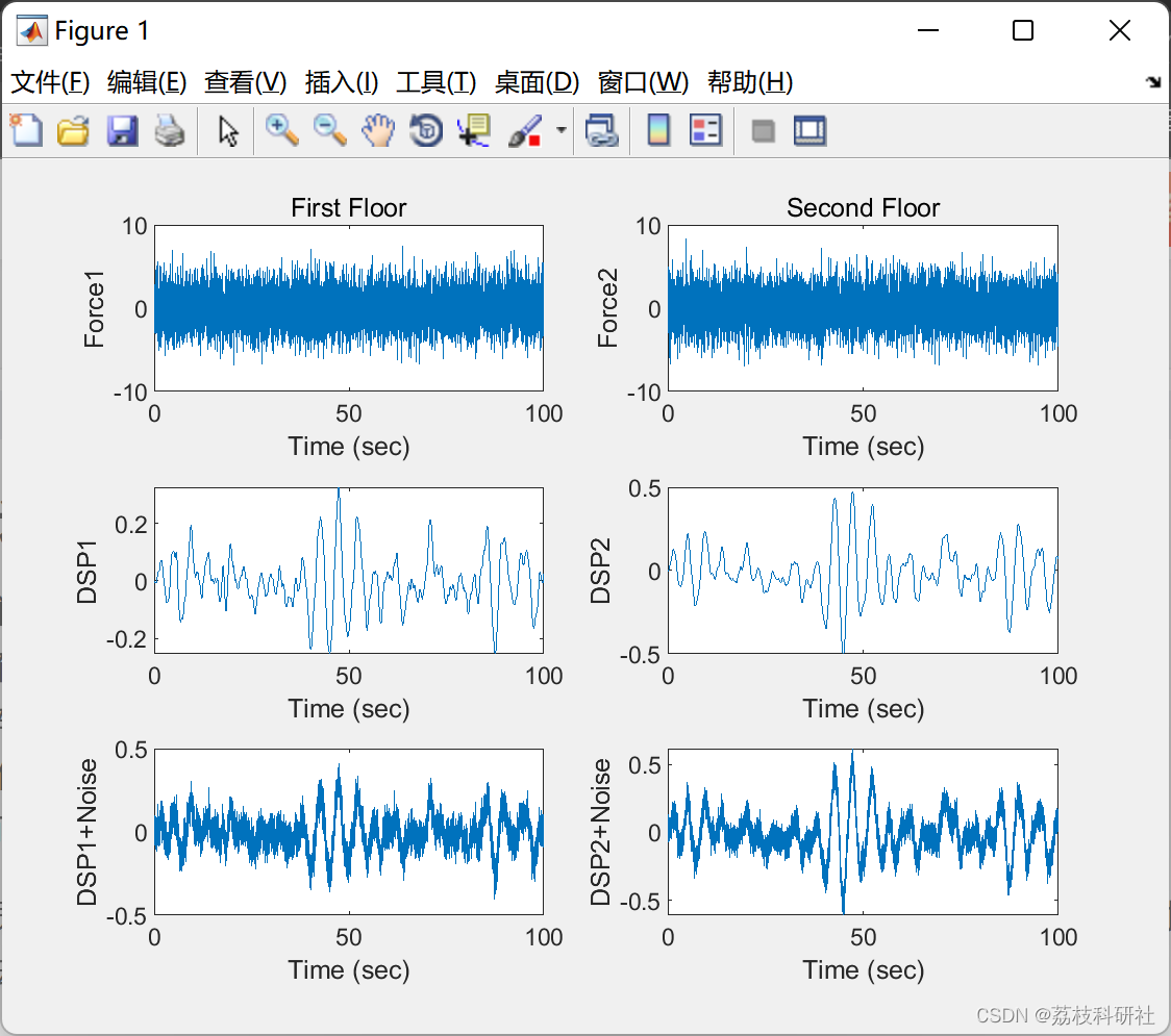
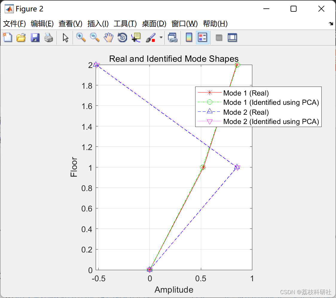
本文使用主成分分析 (PCA) 对 2DOF 系统进行振型识别,该系统受到高斯白噪声激励,并增加了响应的不确定性(也是高斯白噪声)。但是,由于
协方差矩阵的对称性,PCA的特征向量是正颌的。
-模态形状仅在矩阵 inv(M)*K 对称时才是正交的。
-PCA 只有在实振型是正颌时才识别它们,这意味着 inv(M)*K 是对称的。
通过改变质量矩阵M=[2 0; 0 1];而不是恒等式inv(M)*K将不是对称的,即使刚度矩阵是对称的,PCA将无法识别实际的振型。
📚2 运行结果
🌈3 Matlab代码实现
部分代码:
for i=1:1:n
h(i,:)=(1/(Mn(i)*wd(i))).*exp(-zeta(i)*wn(i)*t).*sin(wd(i)*t); %transfer function of displacement
hd(i,:)=(1/(Mn(i)*wd(i))).*(-zeta(i).*wn(i).*exp(-zeta(i)*wn(i)*t).*sin(wd(i)*t)+wd(i).*exp(-zeta(i)*wn(i)*t).*cos(wd(i)*t)); %transfer function of velocity
hdd(i,:)=(1/(Mn(i)*wd(i))).*((zeta(i).*wn(i))^2.*exp(-zeta(i)*wn(i)*t).*sin(wd(i)*t)-zeta(i).*wn(i).*wd(i).*exp(-zeta(i)*wn(i)*t).*cos(wd(i)*t)-wd(i).*((zeta(i).*wn(i)).*exp(-zeta(i)*wn(i)*t).*cos(wd(i)*t))-wd(i)^2.*exp(-zeta(i)*wn(i)*t).*sin(wd(i)*t)); %transfer function of acceleration
qq=conv(fn(i,:),h(i,:))*dt;
qqd=conv(fn(i,:),hd(i,:))*dt;
qqdd=conv(fn(i,:),hdd(i,:))*dt;
q(i,:)=qq(1:steps); % modal displacement
qd(i,:)=qqd(1:steps); % modal velocity
qdd(i,:)=qqdd(1:steps); % modal acceleration
end
x=Vectors*q; %displacement
v=Vectors*qd; %vecloity
a=Vectors*qdd; %vecloity
%Add noise to excitation and response
%--------------------------------------------------------------------------
f2=f+0.05*randn(2,10000);
a2=a+0.05*randn(2,10000);
v2=v+0.05*randn(2,10000);
x2=x+0.05*randn(2,10000);
%Plot displacement of first floor without and with noise
%--------------------------------------------------------------------------
figure;
subplot(3,2,1)
plot(t,f(1,:)); xlabel('Time (sec)'); ylabel('Force1'); title('First Floor');
subplot(3,2,2)
plot(t,f(2,:)); xlabel('Time (sec)'); ylabel('Force2'); title('Second Floor');
subplot(3,2,3)
plot(t,x(1,:)); xlabel('Time (sec)'); ylabel('DSP1');
subplot(3,2,4)
plot(t,x(2,:)); xlabel('Time (sec)'); ylabel('DSP2');
subplot(3,2,5)
plot(t,x2(1,:)); xlabel('Time (sec)'); ylabel('DSP1+Noise');
subplot(3,2,6)
plot(t,x2(2,:)); xlabel('Time (sec)'); ylabel('DSP2+Noise');
%Identify modal parameters using displacement with added uncertainty
%--------------------------------------------------------------------------
[V]=pca(x2'); %PCA eigenvectors
%Plot real and identified first modes to compare between them
%--------------------------------------------------------------------------
figure;
plot([0 ; -Vectors(:,1)],[0 1 2],'r*-');
hold on
plot([0 ;V(:,1)],[0 1 2],'go-.');
hold on
plot([0 ; -Vectors(:,2)],[0 1 2],'b^--');
hold on
plot([0 ;V(:,2)],[0 1 2],'mv:');
hold off
title('Real and Identified Mode Shapes');
legend('Mode 1 (Real)','Mode 1 (Identified using PCA)','Mode 2 (Real)','Mode 2 (Identified using PCA)');
xlabel('Amplitude');
ylabel('Floor');
grid on;
daspect([1 1 1]);
🎉4 参考文献
部分理论来源于网络,如有侵权请联系删除。
[1] Al Rumaithi, Ayad, "Characterization of Dynamic Structures Using Parametric and Non-parametric System Identification Methods" (2014). Electronic Theses and Dissertations. 1325.
[2] Al-Rumaithi, Ayad, Hae-Bum Yun, and Sami F. Masri. "A Comparative Study of Mode Decomposition to Relate Next-ERA, PCA, and ICA Modes." Model Validation and Uncertainty Quantification, Volume 3. Springer, Cham, 2015. 113-133.


 6698
6698


 被折叠的 条评论
为什么被折叠?
被折叠的 条评论
为什么被折叠?
 到【灌水乐园】发言


