机器学习逐渐放弃：SVM

SVM

import numpy as np
import pandas as pd
import sklearn.svm        
import seaborn as sns
import scipy.io as sio  
import matplotlib.pyplot as plt

mat = sio.loadmat('./data/ex6data1.mat')
print(mat.keys())
data = pd.DataFrame(mat.get('X'), columns=['X1', 'X2'])
data['y'] = mat.get('y')

data.head()
>>>
dict_keys(['__header__', '__version__', '__globals__', 'X', 'y'])
          X1	X2	y
0	1.9643	4.5957	1
1	2.2753	3.8589	1
2	2.9781	4.5651	1
3	2.9320	3.5519	1
4	3.5772	2.8560	1


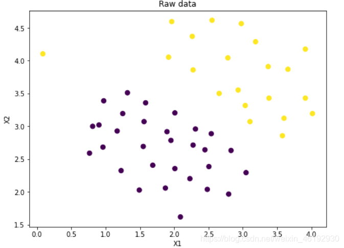
fig, ax = plt.subplots(figsize=(8,6))
ax.scatter(data['X1'], data['X2'], s=50, c=data['y'])   # 散点图，c 是颜色序列
ax.set_title('Raw data')
ax.set_xlabel('X1')
ax.set_ylabel('X2')
plt.show()

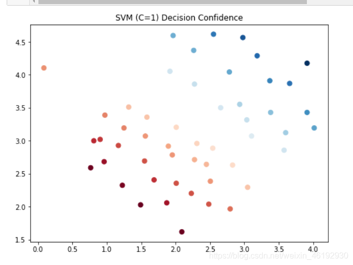
svc1 = sklearn.svm.LinearSVC(C=1, loss='hinge',max_iter = 5000)  # 线性SVM ，hinge 损失函数，
svc1.fit(data[['X1', 'X2']], data['y'])   # C=1，正则化的强度和C 成反比。
svc1.score(data[['X1', 'X2']], data['y'])  # 正确率，，到知识盲区了，，哎
>>> 0.9803921568627451

data['SVM1 Confidence'] = svc1.decision_function(data[['X1', 'X2']])  # 获得样本的置信度评分
fig, ax = plt.subplots(figsize=(8,6))
ax.scatter(data['X1'], data['X2'], s=50, c=data['SVM1 Confidence'], cmap='RdBu')
ax.set_title('SVM (C=1) Decision Confidence')
plt.show()

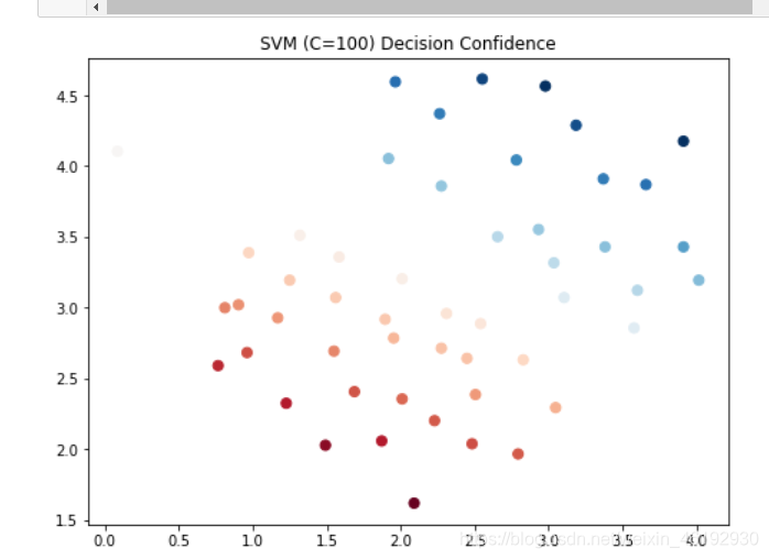
svc100 = sklearn.svm.LinearSVC(C=100, loss='hinge',max_iter=30000)  
svc100.fit(data[['X1', 'X2']], data['y']) # 增加C，最大迭代次数都没啥用啊，，
svc100.score(data[['X1', 'X2']], data['y']) # 为啥评分是一样的呢
>>> 0.9803921568627451


data['SVM100 Confidence'] = svc100.decision_function(data[['X1', 'X2']])
fig, ax = plt.subplots(figsize=(8,6))
ax.scatter(data['X1'], data['X2'], s=50, c=data['SVM100 Confidence'], cmap='RdBu')
ax.set_title('SVM (C=100) Decision Confidence')
plt.show()              # 效果能更好一些

data.head() # 这个置信度分数是到决策边界的有符号距离吧。。
          X1	X2	y	SVM1 Confidence	SVM100 Confidence
0	1.9643	4.5957	1	0.798890	3.847069
1	2.2753	3.8589	1	0.381739	2.012868
2	2.9781	4.5651	1	1.374142	5.045087
3	2.9320	3.5519	1	0.520007	1.919674
4	3.5772	2.8560	1	0.334097	0.634728

加上高斯核

# kernek function 高斯核函数，虽然人家有内置的，但还是来瞅瞅，，
def gaussian_kernel(x1, x2, sigma): # 标准差，决定的是 F 随X 的变化而变化的速率
    return np.exp(- np.power(x1 - x2, 2).sum() / (2 * (sigma ** 2)))

x1 = np.array([1, 2, 1])
x2 = np.array([0, 4, -1])
sigma = 2

gaussian_kernel(x1, x2, sigma)   # x1, x2 应该不算接近了吧。。
>>> 0.32465246735834974


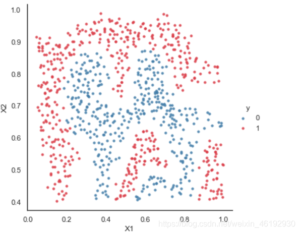
sns.set(context="notebook", style="white", palette=sns.diverging_palette(240, 10, n=2))
sns.lmplot('X1', 'X2', hue='y', data=data,    # 感觉这绘图函数好高级啊，有时间一定要在研究研究
           height=5, 
           fit_reg=False, 
           scatter_kws={"s": 10}
          )
plt.show()    # 这个数据怎么来的，，，

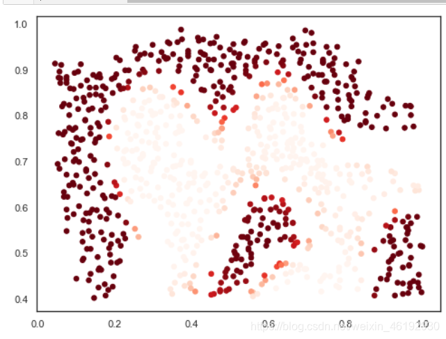
svc = svm.SVC(C=100, kernel='rbf', gamma=10, probability=True) # 使用的核，内核系数，启用概率估计
svc.fit(data[['X1', 'X2']], data['y'])                         # gamma 就是标准差
svc.score(data[['X1', 'X2']], data['y'])
>>> 0.9698725376593279


predict_prob = svc.predict_proba(data[['X1', 'X2']])[:, 1]# 使用这个需要 probability=True，
# 返回样本在模型中每个类的概率，第一列就是类0，第二列就是类1.
fig, ax = plt.subplots(figsize=(8,6))
ax.scatter(data['X1'], data['X2'], s=30, c=predict_prob, cmap='Reds')
plt.show()

寻找最优参数

from sklearn.model_selection import GridSearchCV
from sklearn import metrics

mat = sio.loadmat('./data/ex6data3.mat')
training = pd.DataFrame(mat.get('X'), columns=['X1', 'X2'])
training['y'] = mat.get('y')

cv = pd.DataFrame(mat.get('Xval'), columns=['X1', 'X2'])  # 训练集和交叉验证集
cv['y'] = mat.get('yval')

print(training.shape,cv.shape) 
》》》(211, 3) (200, 3)


candidate = [0.01, 0.03, 0.1, 0.3, 1, 3, 10, 30, 100]
combination = [(C, gamma) for C in candidate for gamma in candidate]
len(combination)  # 9*9，手动构建C 和 gamma（标准差）的网格
>>> 81


search = []
for C, gamma in combination:
    svc = svm.SVC(C=C, gamma=gamma)
    svc.fit(training[['X1', 'X2']], training['y'])     # 使用训练集训练，使用验证机验证。。
    search.append(svc.score(cv[['X1', 'X2']], cv['y']))  # 对不同的C 和gamma计算正确率
best_score = search[np.argmax(search)]
best_param = combination[np.argmax(search)]

print(best_score, best_param)
>>> 0.965 (0.3, 100)

best_svc = svm.SVC(C=100, gamma=0.3)
best_svc.fit(training[['X1', 'X2']], training['y'])
ypred = best_svc.predict(cv[['X1', 'X2']])     # 对新数据（没有训练过的）进行预测

print(metrics.classification_report(cv['y'], ypred)) # 正确率

                  precision    recall  f1-score   support
 
           0       0.92      0.96      0.94       113
           1       0.94      0.89      0.91        87

    accuracy                           0.93       200
   macro avg       0.93      0.92      0.92       200
weighted avg       0.93      0.93      0.92       200

parameters = {'C': candidate, 'gamma': candidate}  # 强大的python连我们手动构建网格都不需要。。
svc = svm.SVC()
clf = GridSearchCV(svc, parameters, n_jobs=-1)
clf.fit(training[['X1', 'X2']], training['y'])                 # 就是调参，，，
print(clf.best_params_,clf.best_score_)
>>> {'C': 30, 'gamma': 3} 0.9194905869324475

ypred = clf.predict(cv[['X1', 'X2']])       
# 结果不一样是因为这个 GridSearchCV 将部分训练集最为验证集去寻找最佳答案
print(metrics.classification_report(cv['y'], ypred)) # 我们手动就用独立的验证集，，感觉还是手动的来的更真实。。
>>>             precision    recall  f1-score   support

           0       0.95      0.96      0.96       113
           1       0.95      0.93      0.94        87

    accuracy                           0.95       200
   macro avg       0.95      0.95      0.95       200
weighted avg       0.95      0.95      0.95       200

• C 过大，高方差，与lambda反着，，
• 标准差过大，高偏差，过小 高方差（过拟合）
• 不使用核函数就是线性核函数
• 当 特征 大于数据 的数量（10倍） 使用logistic or 非线性核 SVM
• 当 n 较小，m 还行 n(1–1000) m(10—10000) 可以使用高斯核SVM
• 当n 小，m 大 n(1–1000) m>50000 需要更多的特征就是用 logistic 或 线性核函数，使用有核的就慢很多。