


本系列所有的代码和数据都可以从陈强老师的个人主页上下载:Python数据程序
参考书目:陈强.机器学习及Python应用. 北京:高等教育出版社, 2021.
本系列基本不讲数学原理,只从代码角度去让读者们利用最简洁的Python代码实现机器学习方法。
聚类分析也是无监督学习,从X里面寻找规律将样本分别归为不同的类。K均值聚类是最常见的聚类法,它运行速度快,适合大数据。分层聚类得到的结果更清晰,但是不合适大数据(运算过慢)
K均值聚类的Python案例
使用模拟数据进行聚类,模拟数据的好处在于我们知道真实的样本的类别
#K-Means Clustering
import numpy as np
import pandas as pd
import matplotlib.pyplot as plt
import seaborn as sns

from sklearn.cluster import KMeans
from sklearn.cluster import AgglomerativeClustering
from sklearn.preprocessing import StandardScaler
from mpl_toolkits.mplot3d import Axes3D
from scipy.cluster.hierarchy import linkage, dendrogram, fcluster
from scipy.spatial.distance import squareform
生成两组数据,可视化
np.random.seed(1)
cluster1 = np.random.normal(0, 1, 100).reshape(-1, 2)
cluster1 = pd.DataFrame(cluster1, columns=['x1', 'x2'])
cluster1['y'] = 0
cluster1.head()

np.random.seed(10)
cluster2 = np.random.normal(3, 1, 100).reshape(-1, 2)
cluster2 = pd.DataFrame(cluster2, columns=['x1', 'x2'])
cluster2['y'] = 1
cluster2.head()

data = pd.concat([cluster1, cluster2])
data.shape

sns.scatterplot(x='x1', y='x2', data=cluster1, color='k', label='y=0')
sns.scatterplot(x='x1', y='x2', data=cluster2, color='b', label='y=1')
plt.legend()
plt.title('True Clusters (K=2)')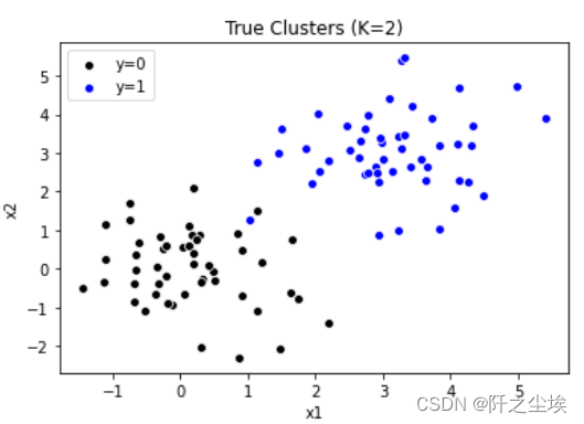
取出X和y,进行K均值聚类
X = data.iloc[:, :-1]
y = data.iloc[:, -1]

model = KMeans(n_clusters=2, random_state=123, n_init=20)
model.fit(X)
#查看聚类标签
model.labels_
#查看聚类中心
model.cluster_centers_
#查看组内平方和
model.inertia_
#画混淆矩阵
pd.crosstab(y, model.labels_, rownames=['Actual'], colnames=['Predicted'])
结果可视化
sns.scatterplot(x='x1', y='x2', data=data[model.labels_ == 0], color='k', label='y=0')
sns.scatterplot(x='x1', y='x2', data=data[model.labels_ == 1], color='b', label='y=1')
plt.legend()
plt.title('Estimated Clusters (K=2)')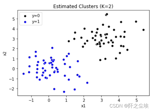
将数据聚为三类
model = KMeans(n_clusters=3, random_state=2, n_init=20)
model.fit(X)

model.labels_
sns.scatterplot(x='x1', y='x2', data=data[model.labels_ == 0], color='k', label='y=0')
sns.scatterplot(x='x1', y='x2', data=data[model.labels_ == 1], color='b', label='y=1')
sns.scatterplot(x='x1', y='x2', data=data[model.labels_ == 2], color='cornflowerblue', label='y=2')
plt.legend()
plt.title('Estimated Clusters (K=3)')
聚类的数目K如何取值,可以使用手肘法判断,即聚类个数K让误差快速下降的位置,则可以取K,误差为mse,手工循环,寻找最优聚类个数K
# Choose optimal K by elbow method
sse = []
for k in range(1,16):
    model = KMeans(n_clusters=k, random_state=1, n_init=20)
    model.fit(X)
    sse.append(model.inertia_)
print(sse)

#画图
plt.plot(range(1, 16), sse, 'o-')
plt.axhline(sse[1], color='k', linestyle='--', linewidth=1)
plt.xlabel('K')
plt.ylabel('SSE')
plt.title('K-means Clustering')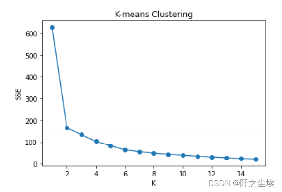
K从1到2下降速度最快,后面没有明显的拐点,k选2最佳
还可以利用AIC个BIC信息准则去挑选(传统统计学方法,如今用得少,效果也不太行)
#AIC
# Choose optimal K by AIC
aic = sse + 2 * 2 * np.arange(1, 16)
aic
min(aic)
np.argmin(aic)
plt.plot(range(1, 16), aic, 'o-')
plt.axvline(np.argmin(aic) + 1, color='k', linestyle='--', linewidth=1)
plt.xlabel('K')
plt.ylabel('AIC')
plt.title('K-means Clustering')

#BIC
# Choose optimal K by BIC
bic = sse + 2 * np.log(100) * np.arange(1, 16)
bic
min(bic)
np.argmin(bic)
plt.plot(range(1, 16), bic, 'o-')
plt.axvline(np.argmin(bic) + 1, color='k', linestyle='--', linewidth=1)
plt.xlabel('K')
plt.ylabel('BIC')
plt.title('K-means Clustering') 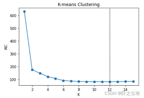
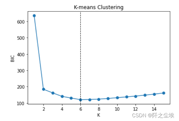
AIC说选12个,BIC说选6个,和真实的2个差的有点远...
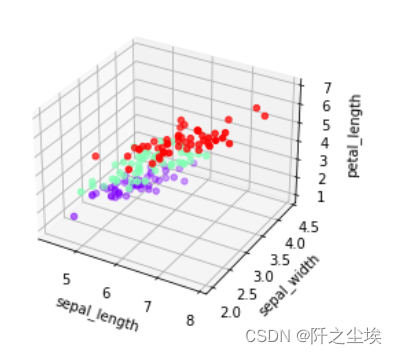
下面采用鸢尾花数据集三个特征变量进行聚类,可以在三维空间图里面可视化
iris = pd.read_csv('iris.csv')
Dict = {'setosa': 0, 'versicolor': 1, 'virginica': 2}
iris.species = iris.species.map(Dict)

fig = plt.figure()
ax = fig.add_subplot(111, projection='3d')
ax.scatter(iris['sepal_length'], iris['sepal_width'],
           iris['petal_length'], c=iris['species'], cmap='rainbow')
ax.set_xlabel('sepal_length')
ax.set_ylabel('sepal_width')
ax.set_zlabel('petal_length')
聚类
# K-means clustering with K=3
X3= iris.iloc[:, :3]
model = KMeans(n_clusters=3, random_state=1, n_init=20)
model.fit(X3)
model.labels_
labels = pd.DataFrame(model.labels_, columns=['label'])
d = {0: 0, 1: 2,2:1}
pred = labels.label.map(d)
table = pd.crosstab(iris.species, pred, rownames=['Actual'], colnames=['Predicted'])
table
accuracy = np.trace(table) / len(iris)
accuracy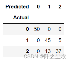 误差不多,聚类结果不错
fig = plt.figure()
ax = fig.add_subplot(111, projection='3d')
ax.scatter(iris['sepal_length'], iris['sepal_width'],
           iris['petal_length'], c=pred, cmap='rainbow')
ax.set_xlabel('sepal_length')
ax.set_ylabel('sepal_width')
ax.set_zlabel('petal_length') 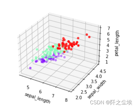
分层聚类Python案例
继续使用鸢尾花数据集,进行不同距离度量的分层聚类。
iris = pd.read_csv('iris.csv')
X = iris.iloc[:, :-1]
X.shape
X.head()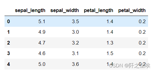 X特征变量
X特征变量
最大值距离
# Complete linkage
linkage_matrix = linkage(X, 'complete')
linkage_matrix.shape

fig = plt.figure(figsize=(16,6))
dendrogram(linkage_matrix)
plt.title('Complete Linkage') 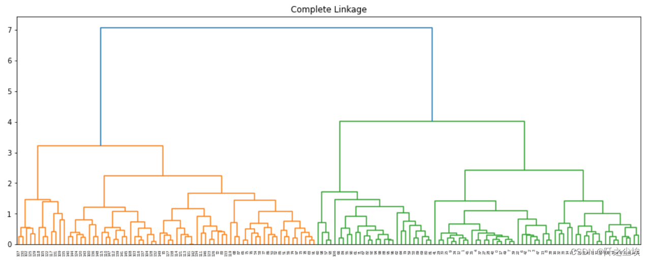
model = AgglomerativeClustering(n_clusters=3, linkage='complete')
model.fit(X)
model.labels_

labels = pd.DataFrame(model.labels_, columns=['label'])
d = {0: 2, 1: 0, 2: 1}
pred = labels['label'].map(d)

table = pd.crosstab(iris.species, pred, rownames=['Actual'], colnames=['Predicted'])
table

accuracy = np.trace(table) / len(iris)
accuracy
#0.84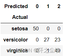
平均距离
# Average linkage
linkage_matrix = linkage(X, 'average')
fig = plt.figure(figsize=(16,6))
dendrogram(linkage_matrix)
plt.title('Average Linkage')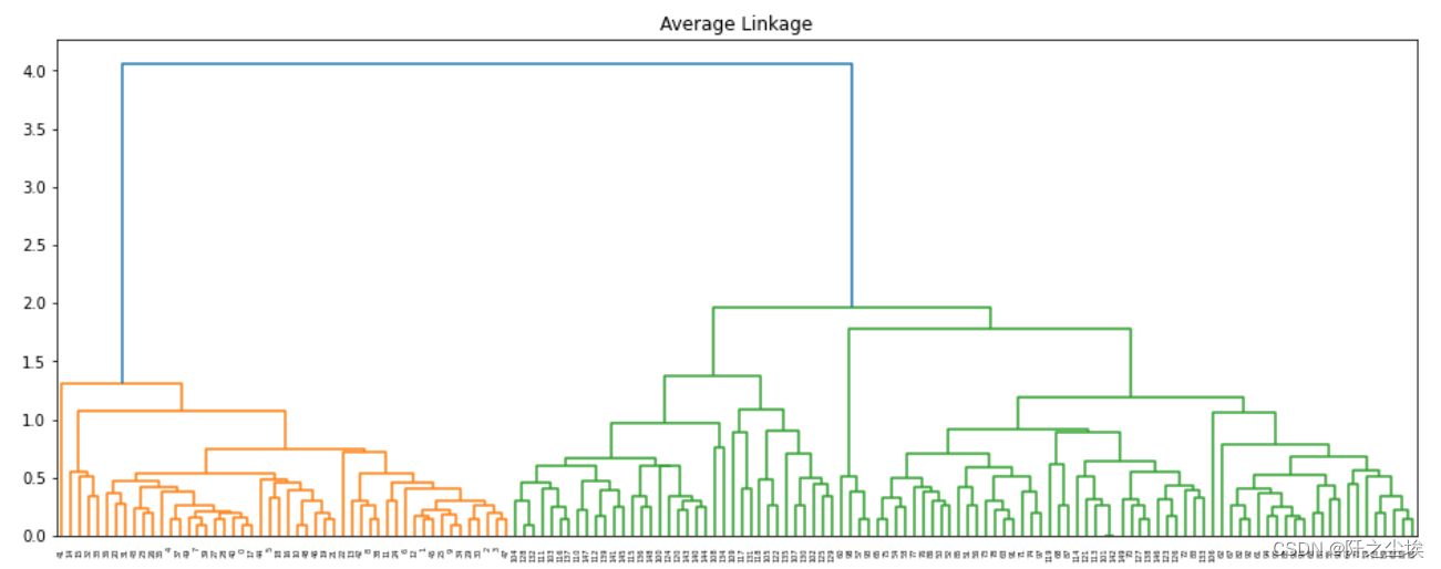
model = AgglomerativeClustering(n_clusters=3, linkage='average')
model.fit(X)
model.labels_
labels = pd.DataFrame(model.labels_, columns=['label'])
d = {0: 1, 1: 0, 2: 2}
pred = labels['label'].map(d)
table = pd.crosstab(iris.species, pred, rownames=['Actual'], colnames=['Predicted'])
table
accuracy = np.trace(table) / len(iris)
accuracy
#0.9066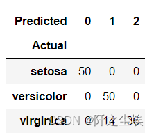
最小距离
# Single linkage

linkage_matrix = linkage(X, 'single')
dendrogram(linkage_matrix)
plt.title('Single Linkage')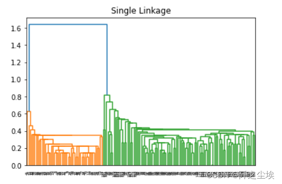
model = AgglomerativeClustering(n_clusters=3, linkage='single')
model.fit(X)

model.labels_
labels = pd.DataFrame(model.labels_, columns=['label'])
d = {0: 1, 1: 0, 2: 2}
pred = labels['label'].map(d)

table = pd.crosstab(iris.species, pred, rownames=['Actual'], colnames=['Predicted'])
table

accuracy = np.trace(table) / len(iris)
accuracy
#0.68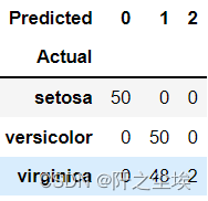
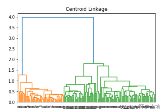
中心距离
# Centroid linkage

linkage_matrix = linkage(X, 'centroid')
dendrogram(linkage_matrix)
plt.title('Centroid Linkage')
labels = fcluster(linkage_matrix, t=3, criterion='maxclust')
labels
labels = pd.DataFrame(labels, columns=['label'])
d = {1: 0, 2: 2, 3: 1}
pred = labels['label'].map(d)
table = pd.crosstab(iris.species, pred, rownames=['Actual'], colnames=['Predicted'])
table
accuracy = np.trace(table) / len(iris)
accuracy
#0.9066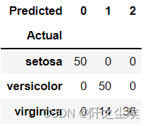
离差平方和
#'ward linkage
linkage_matrix = linkage(X, 'ward')
dendrogram(linkage_matrix)
plt.title('ward Linkage')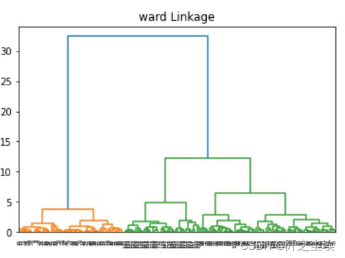
model = AgglomerativeClustering(n_clusters=3, linkage='ward')
model.fit(X)
model.labels_

labels = pd.DataFrame(model.labels_, columns=['label'])
d = {0: 1, 1: 0, 2: 2}
pred = labels['label'].map(d)

table = pd.crosstab(iris.species, pred, rownames=['Actual'], colnames=['Predicted'])
table

accuracy = np.trace(table) / len(iris)
accuracy
#0.89333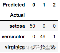
相关系数
## Correlation-based distance measure
dist_matrix = 1 - np.corrcoef(X)
dist_matrix.shape
dist_matrix[:3, :3]
sns.clustermap(dist_matrix, cmap='Blues')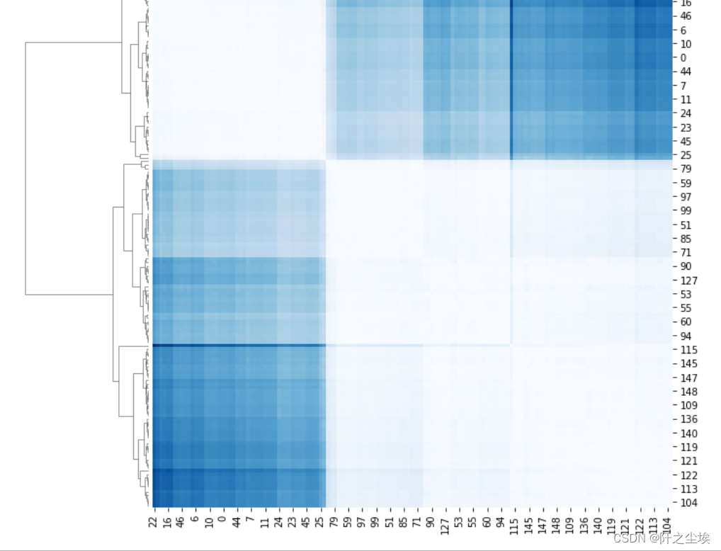
dist = squareform(dist_matrix, checks=False)
dist.shape
linkage_matrix = linkage(dist, 'centroid')
dendrogram(linkage_matrix)
plt.title('Correlated-based Centroid Linkage') 
labels = fcluster(linkage_matrix, t=3, criterion='maxclust')
labels

labels = pd.DataFrame(labels, columns=['label'])
d = {1: 0, 2: 2, 3: 1}
pred = labels['label'].map(d)

table = pd.crosstab(iris.species, pred, rownames=['Actual'], colnames=['Predicted'])
table

accuracy = np.trace(table) / len(iris)
accuracy
#0.94666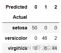
其他聚类方法
from sklearn.preprocessing import StandardScaler
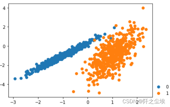
from sklearn.datasets import make_classification
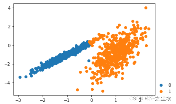
# 原来的综合分类数据集
#from numpy import where
# 定义数据集
X, y = make_classification(n_samples=1000, n_features=2, n_informative=2, n_redundant=0, n_clusters_per_class=1, random_state=4)
# 为每个类的样本创建散点图
for class_value in range(2):
# 获取此类的示例的行索引
row_ix =np.where(y == class_value)
# 创建这些样本的散布
plt.scatter(X[row_ix, 0], X[row_ix, 1])
plt.legend(range(2),frameon=False,bbox_to_anchor=(1, 0), loc=3, borderaxespad=0)
# 绘制散点图
plt.show()
# 亲和力传播聚类
##亲和力传播包括找到一组最能概括数据的范例。
#我们设计了一种名为“亲和传播”的方法,它作为两对数据点之间相似度的输入度量。在数据点之间交换实值消息,直到一组高质量的范例和相应的群集逐渐出现
#它是通过 AffinityPropagation 类实现的,要调整的主要配置是将“ 阻尼 ”设置为0.5到1,甚至可能是“首选项”。

# 定义数据集
from sklearn.cluster import AffinityPropagation
X, _ = make_classification(n_samples=1000, n_features=2, n_informative=2, n_redundant=0, n_clusters_per_class=1, random_state=4)
model = AffinityPropagation(damping=0.9)
model.fit(X)

labels = pd.DataFrame(model.labels_, columns=['label'])
d={0:1,1:0}
#labels.label=labels.label.map(d)

clusters = np.unique(model.labels_)
# 为每个群集的样本创建散点图
for cluster in clusters:
# 获取此群集的示例的行索引
    row_ix = np.where(labels.label== cluster)
    plt.scatter(X[row_ix, 0], X[row_ix, 1])

plt.legend(clusters,frameon=False,bbox_to_anchor=(1, 0), loc=3, borderaxespad=0)
plt.show()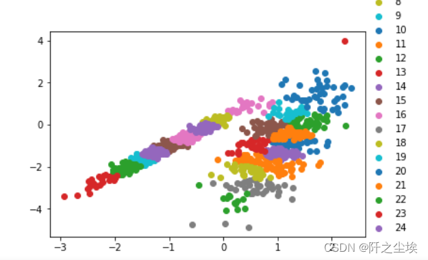
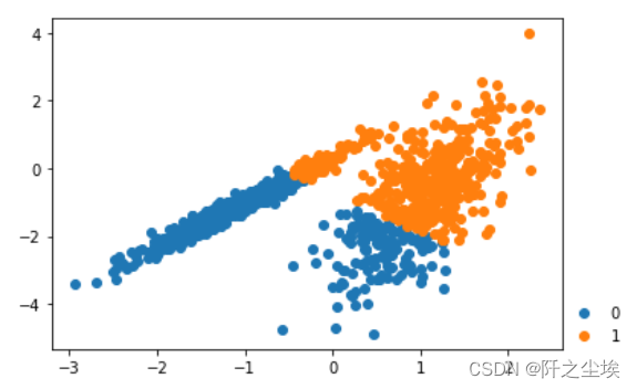
#聚合聚类
#聚合聚类涉及合并示例,直到达到所需的群集数量为止。
#它是层次聚类方法的更广泛类的一部分,通过 AgglomerationClustering 类实现的,主要配置是n _ clusters集,这是对数据中的群集数量的估计。

# 聚合聚类
from sklearn.cluster import AgglomerativeClustering
X, _ = make_classification(n_samples=1000, n_features=2, n_informative=2, n_redundant=0, n_clusters_per_class=1, random_state=4)
model = AgglomerativeClustering(n_clusters=2)
model.fit(X)

labels = pd.DataFrame(model.labels_, columns=['label'])
d={0:1,1:0}
labels.label=labels.label.map(d)

# 检索唯一群集
clusters = np.unique(model.labels_)
# 为每个群集的样本创建散点图
for cluster in clusters:
# 获取此群集的示例的行索引
    row_ix = np.where(labels.label == cluster)
    plt.scatter(X[row_ix, 0], X[row_ix, 1])
plt.legend(clusters,frameon=False,bbox_to_anchor=(1, 0), loc=3, borderaxespad=0)
plt.show()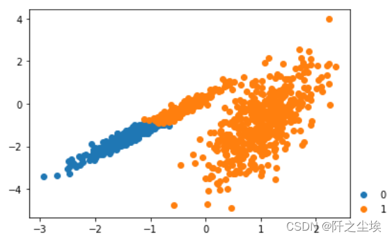
#BIRCH
#BIRCH 聚类( BIRCH 是平衡迭代减少的缩写,聚类使用层次结构)包括构造一个树状结构,从中提取聚类质心。
#BIRCH 递增地和动态地群集传入的多维度量数据点,以尝试利用可用资源(即可用内存和时间约束)产生最佳质量的聚类。
#它是通过 Birch 类实现的,主要配置是“ threshold ”和“ n _ clusters ”超参数,后者提供了群集数量的估计。

# birch聚类
from sklearn.cluster import Birch
# 定义数据集
X, _ = make_classification(n_samples=1000, n_features=2, n_informative=2, n_redundant=0, n_clusters_per_class=1, random_state=4)
model = Birch(threshold=0.01, n_clusters=2)
model.fit(X)

labels = pd.DataFrame(model.labels_, columns=['label'])
d={0:1,1:0}
labels.label=labels.label.map(d)

# 检索唯一群集
clusters = np.unique(model.labels_)
# 为每个群集的样本创建散点图
for cluster in clusters:
# 获取此群集的示例的行索引
    row_ix = np.where(labels.label == cluster)
    plt.scatter(X[row_ix, 0], X[row_ix, 1])
plt.legend(clusters,frameon=False,bbox_to_anchor=(1, 0), loc=3, borderaxespad=0)
plt.show()
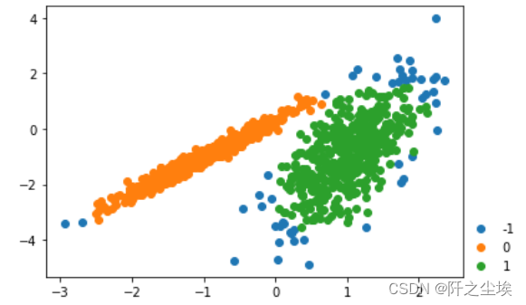
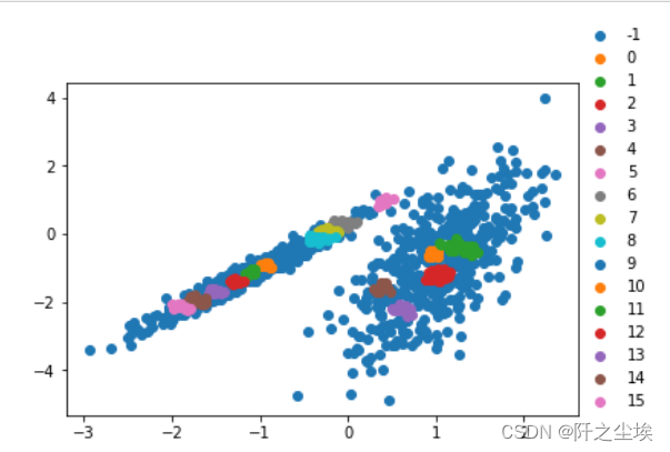
#DBSCAN 聚类(其中 DBSCAN 是基于密度的空间聚类的噪声应用程序)涉及在域中寻找高密度区域,并将其周围的特征空间区域扩展为群集。
#我们提出了新的聚类算法 DBSCAN 依赖于基于密度的概念的集群设计,以发现任意形状的集群。DBSCAN 只需要一个输入参数,并支持用户为其确定适当的值
#它是通过 DBSCAN 类实现的,主要配置是“ eps ”和“ min _ samples ”超参数。

# dbscan 聚类
from sklearn.cluster import DBSCAN
# 定义数据集
X, _ = make_classification(n_samples=1000, n_features=2, n_informative=2, n_redundant=0, n_clusters_per_class=1, random_state=4)

model = DBSCAN(eps=0.30, min_samples=9)
model.fit(X)

labels = pd.DataFrame(model.labels_, columns=['label'])
d={0:1,1:0,-1:-1}
labels.label=labels.label.map(d)
# 检索唯一群集
clusters = np.unique(model.labels_)
# 为每个群集的样本创建散点图
for cluster in clusters:
# 获取此群集的示例的行索引
    row_ix = np.where(labels.label== cluster)
    plt.scatter(X[row_ix, 0], X[row_ix, 1])

plt.legend(clusters,frameon=False,bbox_to_anchor=(1, 0), loc=3, borderaxespad=0)
plt.show()
#Mini-Batch K-均值
#Mini-Batch K-均值是 K-均值的修改版本,它使用小批量的样本而不是整个数据集对群集质心进行更新,这可以使大数据集的更新速度更快,并且可能对统计噪声更健壮。
#我们建议使用 k-均值聚类的迷你批量优化。与经典批处理算法相比,这降低了计算成本的数量级,同时提供了比在线随机梯度下降更好的解决方案。
#它是通过 MiniBatchKMeans 类实现的,要优化的主配置是“ n _ clusters ”超参数,设置为数据中估计的群集数量。


# mini-batch k均值聚类
from sklearn.cluster import MiniBatchKMeans
X, _ = make_classification(n_samples=1000, n_features=2, n_informative=2, n_redundant=0, n_clusters_per_class=1, random_state=4)
model = MiniBatchKMeans(n_clusters=2)
model.fit(X)

labels = pd.DataFrame(model.labels_, columns=['label'])
d={0:1,1:0}
labels.label=labels.label.map(d)

clusters = np.unique(model.labels_)
for cluster in clusters:
    row_ix = np.where(labels.label== cluster)
    plt.scatter(X[row_ix, 0], X[row_ix, 1])

plt.legend(clusters,frameon=False,bbox_to_anchor=(1, 0), loc=3, borderaxespad=0)
plt.show()
#均值漂移聚类
#均值漂移聚类涉及到根据特征空间中的实例密度来寻找和调整质心。
#对离散数据证明了递推平均移位程序收敛到最接近驻点的基础密度函数,从而证明了它在检测密度模式中的应用。
#它是通过 MeanShift 类实现的,主要配置是“带宽”超参数。

# 均值漂移聚类
from sklearn.cluster import MeanShift

# 定义数据集
X, _ = make_classification(n_samples=1000, n_features=2, n_informative=2, n_redundant=0, n_clusters_per_class=1, random_state=4)
# 定义模型
model = MeanShift()
model.fit(X)

labels = pd.DataFrame(model.labels_, columns=['label'])
d={0:1,1:0}
#labels.label=labels.label.map(d)

clusters = np.unique(model.labels_)
for cluster in clusters:
    row_ix = np.where(labels.label== cluster)
    plt.scatter(X[row_ix, 0], X[row_ix, 1])

plt.legend(clusters,frameon=False,bbox_to_anchor=(1, 0), loc=3, borderaxespad=0)
plt.show()

#OPTICS
#OPTICS 聚类( OPTICS 短于订购点数以标识聚类结构)是上述 DBSCAN 的修改版本。
#我们为聚类分析引入了一种新的算法,它不会显式地生成一个数据集的聚类;而是创建表示其基于密度的聚类结构的数据库的增强排序。此群集排序包含相当于密度聚类的信息,该信息对应于范围广泛的参数设置。
#它是通过 OPTICS 类实现的,主要配置是“ eps ”和“ min _ samples ”超参数。

# optics聚类
from sklearn.cluster import OPTICS
X, _ = make_classification(n_samples=1000, n_features=2, n_informative=2, n_redundant=0, n_clusters_per_class=1, random_state=4)
model = OPTICS(eps=0.8, min_samples=10)
model.fit(X)

labels = pd.DataFrame(model.labels_, columns=['label'])
d={0:1,1:0}
#labels.label=labels.label.map(d)

clusters = np.unique(model.labels_)
for cluster in clusters:
    row_ix = np.where(labels.label== cluster)
    plt.scatter(X[row_ix, 0], X[row_ix, 1])

plt.legend(clusters,frameon=False,bbox_to_anchor=(1, 0), loc=3, borderaxespad=0)
plt.show()
#光谱聚类是一类通用的聚类方法,取自线性线性代数。
#最近在许多领域出现的一个有希望的替代方案是使用聚类的光谱方法。这里,使用从点之间的距离导出的矩阵的顶部特征向量。
#它是通过Spectral聚类类实现的,而主要的Spectral聚类是一个由聚类方法组成的通用类,
#取自线性线性代数要优化的是 “n _ clusters” 超参数,用于指定数据中的估计群集数量。

# spectral clustering
from sklearn.cluster import SpectralClustering

X, _ = make_classification(n_samples=1000, n_features=2, n_informative=2, n_redundant=0, n_clusters_per_class=1, random_state=4)
model = SpectralClustering(n_clusters=2)
model.fit(X)

labels = pd.DataFrame(model.labels_, columns=['label'])
d={0:1,1:0}
labels.label=labels.label.map(d)

clusters = np.unique(model.labels_)
for cluster in clusters:
    row_ix = np.where(labels.label== cluster)
    plt.scatter(X[row_ix, 0], X[row_ix, 1])

plt.legend(clusters,frameon=False,bbox_to_anchor=(1, 0), loc=3, borderaxespad=0)
plt.show()
#高斯混合模型
#高斯混合模型总结了一个多变量概率密度函数,顾名思义就是混合了高斯概率分布。
#它是通过 Gaussian Mixture 类实现的,要优化的主要配置是“ n _ clusters ”超参数,用于指定数据中估计的群集数量。

# 高斯混合模型
from sklearn.mixture import GaussianMixture
X, _ = make_classification(n_samples=1000, n_features=2, n_informative=2, n_redundant=0, n_clusters_per_class=1, random_state=4)
model = GaussianMixture(n_components=2)

model.fit(X)
yhat = model.predict(X)

labels = pd.DataFrame(yhat, columns=['label'])
d={0:1,1:0}
labels.label=labels.label.map(d)

clusters = np.unique(yhat)
for cluster in clusters:
    row_ix = np.where(labels.label== cluster)
    plt.scatter(X[row_ix, 0], X[row_ix, 1])

plt.legend(clusters,frameon=False,bbox_to_anchor=(1, 0), loc=3, borderaxespad=0)
plt.show()


 1624
1624


 被折叠的 条评论
为什么被折叠?
被折叠的 条评论
为什么被折叠?
 到【灌水乐园】发言


