Python机器学习20——三十种数据降维方法全面解析（最全数据降维方法总结）

背景

无论是建模还是做科研或者是实际的数据分析中，我们可能面对较多的变量超高维的数据的时候，我们需要用一定的方法去进行降维。这样不仅可以减少数据的冗余，提高计算速度，同时也可以让你的方法显现更多的创新性，以此来忽悠导师，审稿人和领导。

提到数据降维，大部分的人可能只知道做相关性分析，统计学学得好的人还知道逐步回归或者是主成分，因子分析，lasso回归等，机器学习学的好的一点的人可能就会用随机森林，梯度提升等方法去筛选变量重要性。

但是他们对于这些数据的筛选方法，原理以及类别都不太了解。

简单来说，变量筛选可以分为有监督和无监督的，这个很好理解，就是有的变量筛选是需要y的，有的变量筛选是不需要y的，不依靠响应变量y进行变量筛选就是无监督，典型的有因子分析和主成分。而像逐步回归相关性分析或者是lasso回归，随机森林，梯度提升，这些方法都是依赖x和y之间的变量相关性或者重要程度再进行筛选，这些都是有监督的。并且针对不同的分类或者是回归任务所能采用的方法还有所不一样。就比如线性判别分析只能用于分类问题，逐步回归就只能用于回归问题。

但是这种方法其实是很浅显的，本文并不会用这种方法对降维算法来进行分类，我这里使用较为底的数据转化格式的方法进行分类。

本文会依靠不同算法将数据转化的形式将降维方法分为三大类，变量特征选择类，线性特征提取类，非线性特征提取类。

1.变量特征选择类，最好理解的一类，无非就是原来可能有十几个自变量x，我们现在只选出几个重要的x去进行建模，就是从原来很多的特征里面选几个特征去作为新的特征变量X。

典型代表方法例如相关性分析，为了躲避多重共线性的逐步回归，还有加入惩罚项的lasso回归，以及根据变量重要性的随机森林梯度提升类等树模型的集成方法。

2.线性特征提取类，也不难理解，用某种方法把原来的变量的向量映射成了新的一组为向量。而里面的每个都是原来的的线性组合。例如新的变量向量​​​​​​​中的​​​​​​​第一​​​​​​​个​​​​​​​特​​​​​​​征变​​​​​​​量​​​​​​​的取值就是，是原来所有变量的线性组合。具体的这个系数是怎么算的都是根据各个不同的算法来定的。

典型的代表性的方法，如主成分，因子分析，线性判别等。

3.非线性特征提取类，可能这一类方法就有些抽象，因为原来的变量跟降维之后的变量的关系就很难用公式或者是某些函数去进行一个表达。简单来说可以把它看成一个黑箱，你丢十几个x进去会出来几个x，相当于就把x的维度减少了。至于原来的x跟新的x之间是什么关系，我们也不知道。某些方法可以进行一定的可视化和解释性，但是大多数的方法还是不太好解释。

典型的有LLE，ISOMAP，自编码器等方法，这些方法可能大多数人都没听说过，但是他们实现的都挺简单，都是依靠sklearn库就可以了。

为什么要这样分类呢？就主要是因为他们对数据的解释性上有极大的不一样。无论是线性特征提取还是非线性特征提取，他们在转化了x之后，每一个x跟原来的含义都不太一样，其含义就变得很抽象和不可解释，所以在很多业务场景不具有一定的可解释性。大体上人们通常会用的还是去做变量筛选。也就是第一种方法，很多个x里面选几种x作为新的特征变量去建模。

---

方法总结

本文要用的方法总结如下：

变量选择类 这些方法主要关注选择最重要的变量来减少数据维度：

• 方差，异众比例。
• 相关性分析：通过计算变量之间的相关性系数来选择重要特征。
• 计算每个非负特征与类之间的卡方统计量。
• 线性回归（VIF，逐步回归）：使用线性回归模型来评估并选择特征。
• Lasso：通过加罚项进行特征选择。岭回归，弹性网回归。
• 随机森林和梯度提升：使用树模型的重要性度量来选择特征。
• PSI（Population Stability Index）和IV（Information Value）：用于评估特征的稳定性和预测能力。
• SHAP：通过解释模型的输出来评估特征的重要性。

线性特征提取类 这些方法通过线性变换提取特征：

• PCA（主成分分析）：通过协方差矩阵的特征值分解进行降维。
• 增量主成分分析（IPCA）。
• 内核主成分分析（KPCA）通过核技巧扩展PCA以处理非线性数据。
• 稀疏主成分分析（SparsePCA）
• FA（因子分析）：用于发现观测数据中的潜在因子。
• PLS（偏最小二乘回归）：用于回归和分类的降维方法。
• LDA（线性判别分析）：用于分类的降维方法。
• SVD（奇异值分解）：用于矩阵分解和降维。
• 使用截断的SVD（aka LSA）进行降维
• 非负矩阵分解非负矩阵分解（NMF）
• ICA（独立成分分析）：用于从混合信号中提取独立成分。

非线性特征提取类 这些方法适用于非线性数据结构的降维：

• LLE（局部线性嵌入）：保持局部邻域的几何关系。
• LE Laplacian Eigenmaps 是一种非线性降维技术(SpectralEmbedding)
• MDS（多维缩放）：smacof 保留样本间的距离关系。
• t-SNE：特别用于高维数据的可视化，保持局部邻域结构。
• ISOMAP：通过测地距离保持全局结构。
• Autoencoders：神经网络架构，用于学习数据的低维表示。

有的同学数了一下，说你这没有30个哇，骗人退订标题党........因为我很多方法本质上是一类的，但是用的算法不一样，就把它们放到一起了，但实际整体而言，本文给出的降维方法不止30个。

这个总结应该比市面上所有的自媒体都全，并且全部都写成了自定义函数，把原始数据pandas的数据框丢进去就可以返回降维之后的数据框，非常好用。

并且本文也会尝试用一个分类数据集跟一个回归数据集去对比一下，来展示哪些降维方法效果可能会比较好。有的同学可能又要问，不是说有的方法是无监督的吗，那怎么对比效果？无监督只是把x变化了，并不影响我们去用新的x再进行有监督的机器学习。所以下面的整体来说都是遵循这个思路。并且分类问题用准确率，回归问题用拟合优度进行评价测试，我们来评价一下在这些不同的类别任务上，哪些价位方法可能效果会比较好。

回归问题的数集用这个石油价格影响因素，分类问题的数据集就用这个经典的乳腺癌数据集。

---

正文开始，难度是逐一递进的。前面的方法都是最简单的一些学过基础统计的人都会理解的方法。

很多自媒体那些什么根据变量缺失率，变量类型 等进行毫无算法含义的筛选方法都是拿来凑数的。。。本文当然不会放这些浅显简单的方法。

准备数据

导入包

import numpy as np
import pandas as pd
import matplotlib.pyplot as plt 
import seaborn as sns

plt.rcParams ['font.sans-serif'] ='SimHei'               #显示中文
plt.rcParams ['axes.unicode_minus']=False 

读取数据，首先准备我们的这个油价回归的数据集

df_reg=pd.read_excel('降维演示.xlsx',sheet_name='石油回归').set_index('时间')
df_reg.head(2)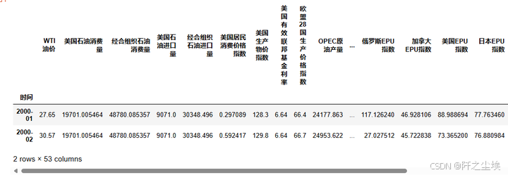

然后再准备乳腺癌的这个分类数据集

df_clf=pd.read_excel('降维演示.xlsx',sheet_name='乳腺癌分类')
df_clf.head(2)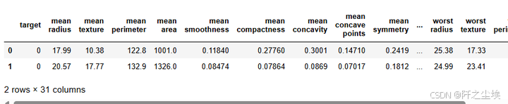

取出x和y查看形状。因为这里只是演示方法，所以说我数据量都比较小。

X_reg=df_reg.drop(columns='WTI油价')
y_reg=df_reg['WTI油价']

X_clf=df_clf.drop(columns='target')
y_clf=df_clf['target']

X_reg.shape,y_reg.shape,X_clf.shape,y_clf.shape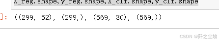

基准效果

我们看看不降维的时候，x对y的这个效果有多少？分类问题跟回归问题分别自定义一个函数，方便复用。

from sklearn.ensemble import RandomForestRegressor, RandomForestClassifier
df_eval_reg=pd.DataFrame(columns=['score'])
df_eval_clf=pd.DataFrame(columns=['score'])

def train_and_evaluate_regressor(X, y,method='原始数据'):
    # 初始化随机森林回归器
    regressor = RandomForestRegressor(  n_estimators=10,max_features=int(X.shape[1]/3), random_state=0)
    # 在数据上进行训练
    regressor.fit(X, y)
    # 在相同数据上进行评分
    score = regressor.score(X, y)
    print(f"回归模型的评分: {score:.4f}")
    df_eval_reg.loc[method]=[score]

def train_and_evaluate_classifier(X, y,method='原始数据'):
    # 初始化随机森林分类器
    classifier = RandomForestClassifier(  n_estimators=10 ,max_features=int(np.sqrt(X.shape[1])),random_state=0)
    # 在数据上进行训练
    classifier.fit(X, y)
    # 在相同数据上进行评分
    score = classifier.score(X, y)
    print(f"分类模型的评分: {score:.4f}")
    df_eval_clf.loc[method]=[score]

计算基础效果：

# 训练和评估
print("回归数据集的X对y的拟合程度：")
train_and_evaluate_regressor(X_reg, y_reg)

print("\n分类数据集的X对y的准确率：")
train_and_evaluate_classifier(X_clf, y_clf)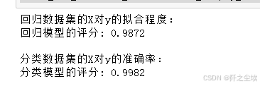

可以看到原始的X对y的解释能力很高。我们降维之后来进行对比。

我们统一降到10维（不好确定个数的方法，我们就将近给他降到10。），看看剩下10个x对于解释能力影响有多大。

---

变量选择类降维

开始进行第一大类的变量降维方法。

方差，异众比例

这个是做数据的初步筛选和清理的时候很常见的方法。因为有的变量他可能取值都很相似，或者取值全部相同，这种变量就没有什么意义了。没有什么区分度，所以我们就会选择删除。而怎么看这些变量的区分度，就可以算变量的方差或者是异众比率。

我们自定义好筛选函数：

from scipy.stats import variation, entropy
def reduce_dimensions_var(x, cv_threshold=0.1, entropy_threshold=0.5):
    """
    根据变异系数或熵值降维数据，并打印保留的列。
    参数:
    - x: pandas DataFrame，输入的数据。
    - cv_threshold: float，变异系数的阈值，低于此值的数值型变量被剔除。
    - entropy_threshold: float，熵值的阈值，高于此值的类别型变量被保留。
    返回:
    - pandas DataFrame，降维后的数据。
    """

    retained_columns = []      # 保留的列
    for column in x.columns:
        if pd.api.types.is_numeric_dtype(x[column]):
            # 计算变异系数
            cv = variation(x[column].dropna())
            if cv > cv_threshold:
                retained_columns.append(column)
        else:
            # 计算熵
            counts = x[column].value_counts(normalize=True)
            ent = entropy(counts)
            if ent > entropy_threshold:
                retained_columns.append(column)

    # 打印保留的列
    print("删除的变量:", set(x.columns)-set(retained_columns))

    # 返回降维后的数据
    return x[retained_columns]

然后运用回归问题上，查看降维之后的x对y的预测效果。

X_reg_rd=reduce_dimensions_var(X_reg, cv_threshold=0.62,)
print(X_reg_rd.shape)
train_and_evaluate_regressor(X_reg_rd, y_reg,method='方差降维')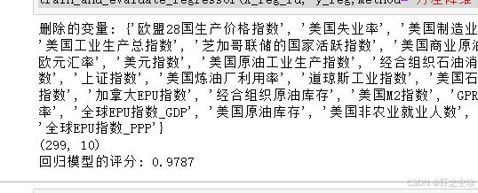

还不错，模型的评分没有下降多少。

分类问题也是一样的：

X_clf_rd=reduce_dimensions_var(X_clf ,cv_threshold=0.62,)
print(X_clf_rd.shape)
train_and_evaluate_classifier(X_clf_rd, y_clf,method='方差降维')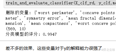

差不多的效果，这些变量对于y的解释能力很强了

---

相关性分析

其实就是看x跟y之间的相关性，这是一个有监督的方法。但是大部分人可能只知道皮尔逊相关性系数。也就是所谓的线性相关，但其实还有很多其他的相关系数：

Pearson（皮尔逊相关系数）： 使用方法：df.corr(method='pearson') 默认方法。 假设数据为正态分布，衡量的是线性相关性。 结果范围为 -1 到 1，0 表示无线性相关性。 Kendall（肯德尔相关系数）： 使用方法：df.corr(method='kendall') 一种基于等级的相关性系数，适合处理有序等级数据。 计算的是两个变量顺序一致性的概率。 Spearman（斯皮尔曼相关系数）： 使用方法：df.corr(method='spearman') 另一种基于等级的相关性系数。 测量的是两个变量的单调关系，即使这种关系不是线性的。

直接上自定义的函数，我们这个函数支持三种相关性系数都可以进行使用，这一下就多了三个降维筛选变量的方法了。

def reduce_dimensions_corr(X, y, method='pearson', num_features=10):
    """
    根据与目标变量的相关性，对特征进行排序，并返回相关性最高的特征。
    
    参数:
    - X: pandas DataFrame，输入的特征数据。
    - y: pandas Series，目标变量。
    - method: str，相关性计算方法，可以是 'pearson'、'kendall' 或 'spearman'。
    - num_features: int，选择的特征数量。
    
    返回:
    - pandas DataFrame，包含选择的特征。
    """
    if method not in ['pearson', 'kendall', 'spearman']:
        raise ValueError("method 参数必须是 'pearson'、'kendall' 或 'spearman'")
    
    # 将目标变量y合并为DataFrame的一列
    data = X.copy() ; data['target'] = y
    # 计算相关性矩阵
    corr_matrix = data.corr(method=method)
    
    # 获取特征与目标之间的相关性（绝对值）
    target_corr = corr_matrix['target'].drop('target').abs()
    
    # 根据相关性排序特征
    sorted_features = target_corr.sort_values(ascending=False).index
    
    # 选择前 num_features 个特征
    selected_features = sorted_features[:num_features]
    
    print(f"选择的特征: {selected_features.tolist()}")
    
    return X[selected_features]

回归问题：

X_reg_rd=reduce_dimensions_corr(X_reg, y_reg, method='pearson', num_features=10)
print(X_reg_rd.shape)
train_and_evaluate_regressor(X_reg_rd, y_reg,method='相关性系数')

分类问题

X_clf_rd=reduce_dimensions_corr(X_clf, y_clf, method='pearson', num_features=10)
print(X_clf_rd.shape)
train_and_evaluate_classifier(X_clf_rd, y_clf,method='相关性系数')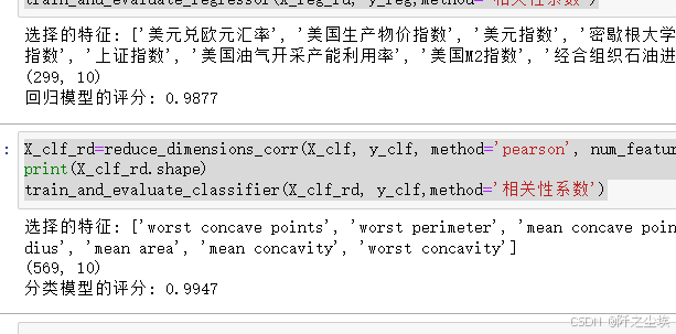

卡方统计量

这个东西有点抽象，可能学过统计学卡方检验才知道这是啥玩意儿，总而言之也是一种根据不同的x研究不同的y的区分度的一个筛选变量的方法。由于他需要y所以这也是一个有监督的方法。

我们上筛选函数，用就行了。

from sklearn.feature_selection import SelectKBest, chi2
def chi_square_feature_selection(X, y, num_features=None):
    """
    使用卡方检验进行特征选择。

    参数:
    - X: pandas DataFrame，包含候选特征。
    - y: pandas Series，目标变量。
    - num_features: int，选择的特征数量（如果为None，则返回所有特征的排序）。

    返回:
    - pandas DataFrame，包含选择的特征。
    """
    # 检查输入数据是否为正数，因为卡方检验要求所有输入数据为正数
    if (X < 0).any().any():
        raise ValueError("X 中的所有特征值必须为非负数。")

    # 初始化卡方检验选择器
    selector = SelectKBest(score_func=chi2, k=num_features)

    # 拟合选择器到数据
    selector.fit(X, y)

    # 获取选择的特征列的索引
    selected_indices = selector.get_support(indices=True)
    selected_features = X.columns[selected_indices]

    print(f"选择的特征: {selected_features.tolist()}")
    return X[selected_features]

分类问题：

X_clf_rd=chi_square_feature_selection(X_clf_rd, y_clf, num_features=10)
print(X_clf_rd.shape)
train_and_evaluate_classifier(X_clf_rd, y_clf,method='卡方统计量')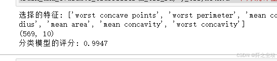

卡方检验只能用于分类问题，回归问题需要用到f统计量检验。

## 回归用F统计量
from sklearn.feature_selection import SelectKBest, f_classif
def f_test_feature_selection(X, y, num_features=None):
    """
    使用F检验（ANOVA F-test）进行特征选择。

    参数:
    - X: pandas DataFrame，包含候选特征。
    - y: pandas Series，目标变量（回归变量）。
    - num_features: int，选择的特征数量（如果为None，则返回所有特征的排序）。

    返回:
    - pandas DataFrame，包含选择的特征。
    """
    # 初始化F检验选择器
    selector = SelectKBest(score_func=f_classif, k=num_features)

    # 拟合选择器到数据
    selector.fit(X, y)

    # 获取选择的特征列的索引
    selected_indices = selector.get_support(indices=True)
    selected_features = X.columns[selected_indices]

    print(f"选择的特征: {selected_features.tolist()}")
    return X[selected_features]

X_reg_rd=f_test_feature_selection(X_reg, y_reg, num_features=10)
print(X_reg_rd.shape)
train_and_evaluate_regressor(X_reg_rd, y_reg,method='F统计量')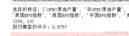

效果感觉不太行。

---

线性回归

其实就是逐步回归，根据一些前项选择，后项选择来筛选变量。

import statsmodels.api as sm
def forward_selection(X, y, significance_level=0.05):
    """
    使用前向选择法来选择特征。

    参数:
    - X: pandas DataFrame，包含候选特征。
    - y: pandas Series，目标变量。
    - significance_level: float，显著性水平。

    返回:
    - pandas DataFrame，包含选择的特征。
    """
    initial_features = X.columns.tolist()
    best_features = []
    
    while len(initial_features) > 0:
        remaining_features = list(set(initial_features) - set(best_features))
        new_pval = pd.Series(index=remaining_features, dtype=float)  # 指定数据类型以避免警告
        for new_column in remaining_features:
            model = sm.OLS(y, sm.add_constant(X[best_features + [new_column]])).fit()
            new_pval[new_column] = model.pvalues[new_column]
        min_p_value = new_pval.min()
        if min_p_value < significance_level:
            best_features.append(new_pval.idxmin())
        else:
            break
    
    print(f"选择的特征: {best_features}")
    return X[best_features]

使用：

X_reg_rd=forward_selection(X_reg, y_reg, significance_level=0.01)
print(X_reg_rd.shape)
train_and_evaluate_regressor(X_reg_rd, y_reg,method='逐步回归')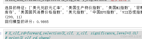

因为是回归问题嘛，所以说分类数据这里就用不了这个方法。

下面的拉索岭回归，岭回归，弹性网回归都用不了分类，都只适用于回归问题去进行变量筛选。

---

Lasso回归，岭回归，弹性网回归

这三类方法为什么我要放一起？就是因为他们都是基于乘惩罚项进行变量筛选。只是惩罚项的形式有些不一样。

首先是Lasso回归

## lasso回归
from sklearn.linear_model import Lasso
from sklearn.preprocessing import StandardScaler

def lasso_feature_selection(X, y, alpha=1.0, num_features=None):
    """
    使用Lasso回归进行特征选择。

    参数:
    - X: pandas DataFrame，包含候选特征。
    - y: pandas Series，目标变量。
    - alpha: float，Lasso回归中的正则化强度参数。
    - num_features: int，选择的特征数量（可选）。

    返回:
    - pandas DataFrame，包含选择的特征。
    """
    # 标准化特征
    scaler = StandardScaler()
    X_scaled = scaler.fit_transform(X)

    # 创建Lasso回归模型并拟合数据
    lasso = Lasso(alpha=alpha, random_state=42)
    lasso.fit(X_scaled, y)

    # 获取系数非零的特征
    coef = lasso.coef_
    selected_indices = [i for i, c in enumerate(coef) if c != 0]
    selected_features = X.columns[selected_indices]

    # 如果指定了特征数量，则选择前num_features个特征
    if num_features is not None:
        selected_features = selected_features[:num_features]

    print(f"选择的特征: {selected_features.tolist()}")
    return X[selected_features]

使用：

X_reg_rd=lasso_feature_selection(X_reg, y_reg, num_features=10)
print(X_reg_rd.shape)
train_and_evaluate_regressor(X_reg_rd, y_reg,method='lasso回归')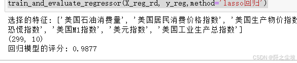

岭回归：

## 岭回归回归
from sklearn.linear_model import Ridge
def ridge_feature_selection(X, y, alpha=1.0, num_features=None):
    """
    使用岭回归对特征进行排序并选择最重要的特征。

    参数:
    - X: pandas DataFrame，包含候选特征。
    - y: pandas Series，目标变量。
    - alpha: float，岭回归中的正则化强度参数。
    - num_features: int，选择的特征数量（可选）。

    返回:
    - pandas DataFrame，包含选择的特征。
    """
    # 标准化特征
    scaler = StandardScaler()
    X_scaled = scaler.fit_transform(X)

    # 创建岭回归模型并拟合数据
    ridge = Ridge(alpha=alpha, random_state=42)
    ridge.fit(X_scaled, y)

    # 获取系数的绝对值并排序
    coef = np.abs(ridge.coef_)
    sorted_indices = np.argsort(coef)[::-1]  # 从大到小排序
    selected_features = X.columns[sorted_indices]

    # 如果指定了特征数量，则选择前num_features个特征
    if num_features is not None:
        selected_features = selected_features[:num_features]

    print(f"选择的特征: {selected_features.tolist()}")
    return X[selected_features]

 使用：

X_reg_rd=ridge_feature_selection(X_reg, y_reg, num_features=10)
print(X_reg_rd.shape)
train_and_evaluate_regressor(X_reg_rd, y_reg,method='岭回归')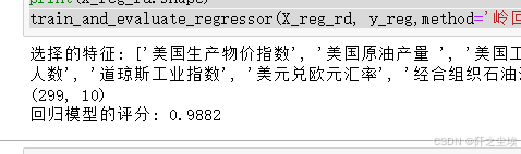

弹性网回归

## 弹性网回归
from sklearn.linear_model import ElasticNet
def elastic_net_feature_selection(X, y, alpha=1.0, l1_ratio=0.5, num_features=None):
    """
    使用弹性网回归对特征进行选择。

    参数:
    - X: pandas DataFrame，包含候选特征。
    - y: pandas Series，目标变量。
    - alpha: float，弹性网中的正则化强度参数。
    - l1_ratio: float，L1范数的比例，0表示Ridge，1表示Lasso。
    - num_features: int，选择的特征数量（可选）。

    返回:
    - pandas DataFrame，包含选择的特征。
    """
    # 标准化特征
    scaler = StandardScaler()
    X_scaled = scaler.fit_transform(X)

    # 创建弹性网回归模型并拟合数据
    elastic_net = ElasticNet(alpha=alpha, l1_ratio=l1_ratio, random_state=42)
    elastic_net.fit(X_scaled, y)

    # 获取系数的绝对值并排序
    coef = np.abs(elastic_net.coef_)
    sorted_indices = np.argsort(coef)[::-1]  # 从大到小排序
    selected_features = X.columns[sorted_indices]

    # 如果指定了特征数量，则选择前num_features个特征
    if num_features is not None:
        selected_features = selected_features[:num_features]

    print(f"选择的特征: {selected_features.tolist()}")
    return X[selected_features]

使用

X_reg_rd=elastic_net_feature_selection(X_reg, y_reg, num_features=10)
print(X_reg_rd.shape)
train_and_evaluate_regressor(X_reg_rd, y_reg,method='弹性网回归')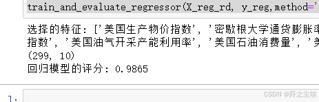

上面这些方法基本都是传统统计学的一些基于线性模型的方法，下面使用机器学习的树模型的方法。

---

决策树、 随机森林和梯度提升

关于为什么决策树以及它衍生出来的集成模型可以进行变量筛选的原理。主要是其构建损失函数的时候，在变量分裂往下进行叶子节点的衍生时，会让损失函数的下降幅度程度不一样，程度越大说明这个变量越重要。具体原理可以网上去搜一搜，或者问一下AI。这里主要是教大家如何使用。并且这些机器学习的非线性的模型无论是使用于回归问题还是分类问题都是可以的，效果也很好，所以说很好用。基本上实际生活生产作业论文中我用的都是这些方法。上面那些lasso回归什么的，忽悠上个世纪的老教授和古板的审稿人还差不多。

决策树

from sklearn.tree import DecisionTreeRegressor, DecisionTreeClassifier
def decision_tree_feature_selection(X, y, task_type='reg', num_features=None, max_depth=None):
    """
    使用决策树进行特征选择。

    参数:
    - X: pandas DataFrame，包含候选特征。
    - y: pandas Series，目标变量。
    - task_type: str，任务类型，'reg' 或 'clf'。
    - num_features: int，选择的特征数量（如果为None，则返回所有特征的排序）。
    - max_depth: int，决策树的最大深度（可选）。

    返回:
    - pandas DataFrame，包含选择的特征。
    """
    # 根据任务类型选择模型
    if task_type == 'reg':
        model = DecisionTreeRegressor(max_depth=max_depth, random_state=42)
    elif task_type == 'clf':
        model = DecisionTreeClassifier(max_depth=max_depth, random_state=42)
    else:
        raise ValueError("task_type 参数必须是 'reg' 或 'clf'")

    # 拟合模型
    model.fit(X, y)

    # 获取特征重要性并排序
    importances = model.feature_importances_
    sorted_indices = np.argsort(importances)[::-1]  # 从大到小排序
    selected_features = X.columns[sorted_indices]

    # 如果指定了特征数量，则选择前num_features个特征
    if num_features is not None:
        selected_features = selected_features[:num_features]

    print(f"选择的特征: {selected_features.tolist()}")
    return X[selected_features]

回归使用

X_reg_rd=decision_tree_feature_selection(X_reg, y_reg, task_type='reg', num_features=10)
print(X_reg_rd.shape)
train_and_evaluate_regressor(X_reg_rd, y_reg,method='决策树')

分类

X_clf_rd=decision_tree_feature_selection(X_clf, y_clf, task_type='clf', num_features=10)
print(X_clf_rd.shape)
train_and_evaluate_classifier(X_clf_rd, y_clf,method='决策树')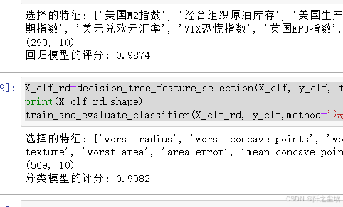

随机森林

## 随机森林
from sklearn.ensemble import RandomForestRegressor, RandomForestClassifier
def random_forest_feature_selection(X, y, task_type='reg', num_features=None, n_estimators=100):
    """
    使用随机森林进行特征选择。
    参数:
    - X: pandas DataFrame，包含候选特征。
    - y: pandas Series，目标变量。
    - task_type: str，任务类型，'reg' 或 'clf'。
    - num_features: int，选择的特征数量（如果为None，则返回所有特征的排序）。
    - n_estimators: int，随机森林中的树的数量。

    返回:
    - pandas DataFrame，包含选择的特征。
    """
    # 根据任务类型选择模型
    if task_type == 'reg':
        rf = RandomForestRegressor(n_estimators=n_estimators, random_state=42)
    elif task_type == 'clf':
        rf = RandomForestClassifier(n_estimators=n_estimators, random_state=42)
    else:
        raise ValueError("task_type 参数必须是 'reg' 或 'clf'")

    # 拟合模型
    rf.fit(X, y)

    # 获取特征重要性并排序
    importances = rf.feature_importances_
    sorted_indices = np.argsort(importances)[::-1]  # 从大到小排序
    selected_features = X.columns[sorted_indices]

    # 如果指定了特征数量，则选择前num_features个特征
    if num_features is not None:
        selected_features = selected_features[:num_features]

    print(f"选择的特征: {selected_features.tolist()}")
    return X[selected_features]

回归

X_reg_rd=random_forest_feature_selection(X_reg, y_reg, task_type='reg', num_features=10)
print(X_reg_rd.shape)
train_and_evaluate_regressor(X_reg_rd, y_reg,method='随机森林')

分类：

X_clf_rd=random_forest_feature_selection(X_clf, y_clf, task_type='clf', num_features=10)
print(X_clf_rd.shape)
train_and_evaluate_classifier(X_clf_rd, y_clf,method='随机森林')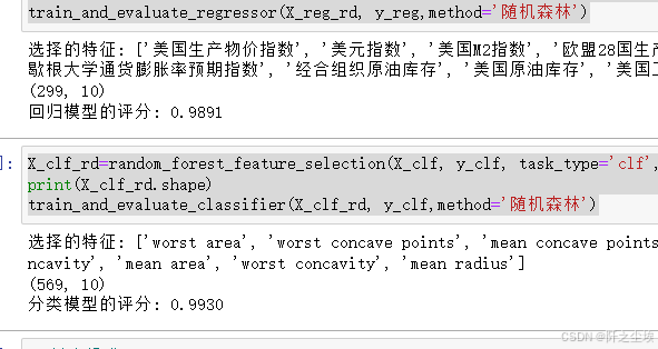

 

梯度提升

##梯度提升
from sklearn.ensemble import GradientBoostingRegressor, GradientBoostingClassifier
def gradient_boosting_feature_selection(X, y, task_type='reg', num_features=None, n_estimators=100):
    """
    使用梯度提升进行特征选择。
    参数:
    - X: pandas DataFrame，包含候选特征。
    - y: pandas Series，目标变量。
    - task_type: str，任务类型，'reg' 或 'clf'。
    - num_features: int，选择的特征数量（如果为None，则返回所有特征的排序）。
    - n_estimators: int，梯度提升中的树的数量。

    返回:
    - pandas DataFrame，包含选择的特征。
    """
    # 根据任务类型选择模型
    if task_type == 'reg':
        model = GradientBoostingRegressor(n_estimators=n_estimators, random_state=42)
    elif task_type == 'clf':
        model = GradientBoostingClassifier(n_estimators=n_estimators, random_state=42)
    else:
        raise ValueError("task_type 参数必须是 'reg' 或 'clf'")

    # 拟合模型
    model.fit(X, y)

    # 获取特征重要性并排序
    importances = model.feature_importances_
    sorted_indices = np.argsort(importances)[::-1]  # 从大到小排序
    selected_features = X.columns[sorted_indices]

    # 如果指定了特征数量，则选择前num_features个特征
    if num_features is not None:
        selected_features = selected_features[:num_features]

    print(f"选择的特征: {selected_features.tolist()}")
    return X[selected_features]

回归

X_reg_rd=gradient_boosting_feature_selection(X_reg, y_reg, task_type='reg', num_features=10)
print(X_reg_rd.shape)
train_and_evaluate_regressor(X_reg_rd, y_reg,method='梯度提升')

分类

X_clf_rd=gradient_boosting_feature_selection(X_clf, y_clf, task_type='clf', num_features=10)
print(X_clf_rd.shape)
train_and_evaluate_classifier(X_clf_rd, y_clf,method='梯度提升')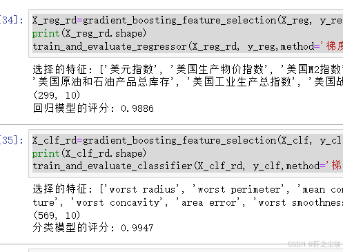

XGboost

如果说你做机器学习还不知道XGboost和LGBM这些基于梯度提升改进的模型，那我只能说你机器学习还没入门......实在不知道的话去搜一下，看我之前的文章也行。没有这个库记得装一下

### xgboost提取
from xgboost import XGBRegressor, XGBClassifier
def xgboost_feature_selection(X, y, task_type='reg', num_features=None, n_estimators=100):
    """
    使用XGBoost进行特征选择。
    参数:
    - X: pandas DataFrame，包含候选特征。
    - y: pandas Series，目标变量。
    - task_type: str，任务类型，'reg' 或 'clf'。
    - num_features: int，选择的特征数量（如果为None，则返回所有特征的排序）。
    - n_estimators: int，XGBoost中的树的数量。

    返回:
    - pandas DataFrame，包含选择的特征。
    """
    # 根据任务类型选择模型
    if task_type == 'reg':
        model = XGBRegressor(n_estimators=n_estimators, random_state=0)
    elif task_type == 'clf':
        model = XGBClassifier(n_estimators=n_estimators,random_state=0, use_label_encoder=False)
    else:
        raise ValueError("task_type 参数必须是 'reg' 或 'clf'")

    # 拟合模型
    model.fit(X, y)

    # 获取特征重要性并排序
    importances = model.feature_importances_
    sorted_indices = np.argsort(importances)[::-1]  # 从大到小排序
    selected_features = X.columns[sorted_indices]

    # 如果指定了特征数量，则选择前num_features个特征
    if num_features is not None:
        selected_features = selected_features[:num_features]

    print(f"选择的特征: {selected_features.tolist()}")
    return X[selected_features]

回归

X_reg_rd=xgboost_feature_selection(X_reg, y_reg, task_type='reg', num_features=10)
print(X_reg_rd.shape)
train_and_evaluate_regressor(X_reg_rd, y_reg,method='XGboost')

分类

X_clf_rd=xgboost_feature_selection(X_clf, y_clf, task_type='clf', num_features=10)
print(X_clf_rd.shape)
train_and_evaluate_classifier(X_clf_rd, y_clf,method='XGboost')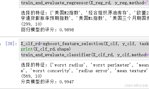

LGBM

也是一样的，没有这个库记得装一下。

from lightgbm import LGBMRegressor, LGBMClassifier
def lightgbm_feature_selection(X, y, task_type='reg', num_features=None, n_estimators=100):
    """
    使用LightGBM进行特征选择。
    参数:
    - X: pandas DataFrame，包含候选特征。
    - y: pandas Series，目标变量。
    - task_type: str，任务类型，'reg' 或 'clf'。
    - num_features: int，选择的特征数量（如果为None，则返回所有特征的排序）。
    - n_estimators: int，LightGBM中的树的数量。

    返回:
    - pandas DataFrame，包含选择的特征。
    """
    # 根据任务类型选择模型
    if task_type == 'reg':
        model = LGBMRegressor(n_estimators=n_estimators, random_state=42)
    elif task_type == 'clf':
        model = LGBMClassifier(n_estimators=n_estimators, random_state=42)
    else:
        raise ValueError("task_type 参数必须是 'reg' 或 'clf'")

    # 拟合模型
    model.fit(X, y)

    # 获取特征重要性并排序
    importances = model.feature_importances_
    sorted_indices = np.argsort(importances)[::-1]  # 从大到小排序
    selected_features = X.columns[sorted_indices]

    # 如果指定了特征数量，则选择前num_features个特征
    if num_features is not None:
        selected_features = selected_features[:num_features]

    print(f"选择的特征: {selected_features.tolist()}")
    return X[selected_features]

使用

X_reg_rd=lightgbm_feature_selection(X_reg, y_reg, task_type='reg', num_features=10)
print(X_reg_rd.shape)
train_and_evaluate_regressor(X_reg_rd, y_reg,method='LGBM')
X_clf_rd=lightgbm_feature_selection(X_clf, y_clf, task_type='clf', num_features=10)
print(X_clf_rd.shape)
train_and_evaluate_classifier(X_clf_rd, y_clf,method='LGBM')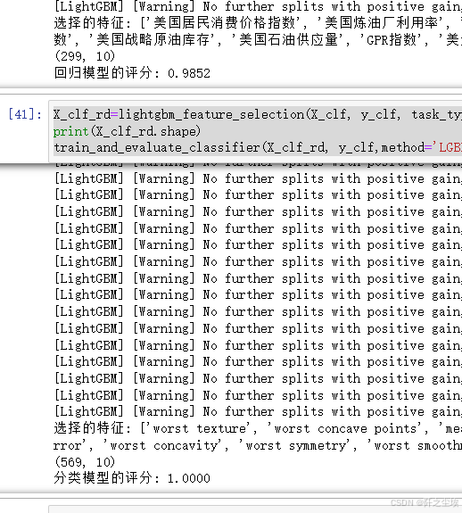

PSI和IV筛选

这两个方法主要是在信贷场景的机器学习用的比较多。PSI是无监督的，主要是依赖于变量的稳定性进行一个筛选。Iv主要是针对2分类问题进行筛选，并且其手算写函数有点复杂，可以借助一些包。

IV筛选

# import scorecardpy as sc
# dt_s = sc.var_filter(pd.concat([X_clf,y_clf],axis=1), y="target",iv_limit=0.02, missing_limit=0.95, identical_limit=0.95,return_rm_reason=True)
# X_clf_rd=dt_s['dt']
# print(X_clf_rd.shape)
# train_and_evaluate_classifier(X_clf_rd, y_clf,method='iv选择')

这里就不运行演示了，因为这个方法不是很通用，只能在2分类问题才能用。

PSI筛选

#PSI计算筛选
def calculate_psi(expected_array, actual_array, buckets=10):
    """计算单个特征的PSI值"""
    def scale_range(input, min, max):
        input += -(np.min(input))
        input /= np.max(input) / (max - min)
        input += min
        return input

    breakpoints = np.arange(0, buckets + 1) / buckets * 100
    expected_percents = np.percentile(expected_array, breakpoints)
    actual_percents = np.percentile(actual_array, breakpoints)
    
    expected_counts = np.histogram(expected_array, bins=expected_percents)[0]
    actual_counts = np.histogram(actual_array, bins=actual_percents)[0]
    
    expected_probs = expected_counts / len(expected_array)
    actual_probs = actual_counts / len(actual_array)
    
    psi_values = (expected_probs - actual_probs) * np.log(expected_probs / actual_probs)
    psi_values = np.where(np.isnan(psi_values), 0, psi_values)  # 防止NaN
    psi = np.sum(psi_values)
    
    return psi

def filter_features_by_psi(X, psi_threshold=0.1, train_size=0.8):
    """根据PSI筛选特征"""
    # 计算训练集的大小
    train_count = int(len(X) * train_size)
    train_data = X[:train_count]
    test_data = X[train_count:]
    
    selected_features = []
    
    for column in X.columns:
        train_array = train_data[column].to_numpy()
        test_array = test_data[column].to_numpy()
        psi_value = calculate_psi(train_array, test_array)
        
        # 只保留PSI小于阈值的特征
        if psi_value <= psi_threshold:
            selected_features.append(column)
    
    return X[selected_features]

使用

X_reg_rd=filter_features_by_psi(X_reg ,psi_threshold=0.0001602665,)
print(X_reg_rd.shape)
train_and_evaluate_regressor(X_reg_rd, y_reg,method='PSI')
X_clf_rd=filter_features_by_psi(X_clf, psi_threshold=0.001953,)
print(X_clf_rd.shape)
train_and_evaluate_classifier(X_clf_rd, y_clf,method='PSI')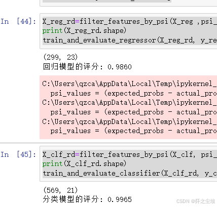

这里太难控制将变量筛选变成10个了，所以就20多个吧，反正效果也差不多。

SHAP：通过解释模型的输出来评估特征的重要性

shap这个库可以说是解决了很多机器学习黑商问题，没有办法解释的痛点，其也是依据一些方法来评估每个变量对于模型的重要性。当然要计算shap之前我们得先训练一个模型，我们这里就采用最常用的LGbm模型进行训练，然后采用夏普包进行一个特征筛选和评价。

from lightgbm import LGBMRegressor, LGBMClassifier
import shap

def shap_feature_selection(X, y, task_type='reg', num_features=None, n_estimators=100):
    """
    使用SHAP进行特征选择。
    参数:
    - X: pandas DataFrame，包含候选特征。
    - y: pandas Series，目标变量。
    - task_type: str，任务类型，'reg' 或 'clf'。
    - num_features: int，选择的特征数量（如果为None，则返回所有特征的排序）。
    - n_estimators: int，LightGBM中的树的数量。

    返回:
    - pandas DataFrame，包含选择的特征。
    """
    # 根据任务类型选择模型
    if task_type == 'reg':
        model = LGBMRegressor(n_estimators=n_estimators, random_state=0)
    elif task_type == 'clf':
        model = LGBMClassifier(n_estimators=n_estimators, random_state=0)
    else:
        raise ValueError("task_type 参数必须是 'reg' 或 'clf'")

    # 拟合模型
    model.fit(X, y)

    # 使用 SHAP 计算特征重要性
    explainer = shap.Explainer(model, X)
    shap_values = explainer(X)
    
    # 计算特征重要性（平均绝对SHAP值）
    shap_importances = np.abs(shap_values.values).mean(axis=0)
    sorted_indices = np.argsort(shap_importances)[::-1]  # 从大到小排序
    selected_features = X.columns[sorted_indices]

    # 如果指定了特征数量，则选择前num_features个特征
    if num_features is not None:
        selected_features = selected_features[:num_features]

    print(f"选择的特征: {selected_features.tolist()}")
    return X[selected_features]

使用：

X_reg_rd=shap_feature_selection(X_reg, y_reg, task_type='reg', num_features=10)
print(X_reg_rd.shape)
train_and_evaluate_regressor(X_reg_rd, y_reg,method='Shap')
X_clf_rd=shap_feature_selection(X_clf, y_clf, task_type='clf', num_features=10)
print(X_clf_rd.shape)
train_and_evaluate_classifier(X_clf_rd, y_clf,method='Shap')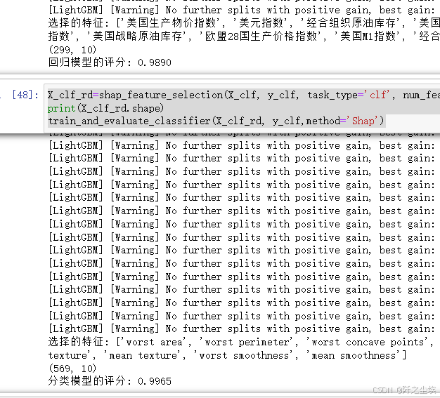

我觉得效果还是挺不错的。

---

线性特征提取类

下面到了第二大类的特征降维的方法了，也是一样，方法从最耳熟能详的主成分到一些比较复杂的方法。

主成分类

主成分类的方法有太多了，有最普通的主成分，增量主成分，内核主成分，稀疏主成分，我们下面把它都写入一个函数，用一个参数来进行选择，反正都是差不多的。

from sklearn.decomposition import PCA, IncrementalPCA, SparsePCA,KernelPCA

def pca_dimensionality_reduction(X, method='PCA', num_components=None, kernel='linear'):
    """
    使用指定的降维方法进行降维。
    
    参数:
    - X: pandas DataFrame，包含原始特征。
    - method: str，降维方法，'PCA'、'IPCA'、'KPCA'、'SparsePCA'。
    - num_components: int，选择的主成分数量（如果为None，则保留所有主成分）。
    - kernel: str，KPCA方法中使用的核类型，仅在使用KPCA时有效。
    
    返回:
    - pandas DataFrame，包含降维后的数据。
    """
    if method == 'PCA':
        model = PCA(n_components=num_components, random_state=0)
    elif method == 'IPCA':
        model = IncrementalPCA(n_components=num_components)
    elif method == 'KPCA':
        model = KernelPCA(n_components=num_components, kernel=kernel, fit_inverse_transform=True, random_state=0)
    elif method == 'SparsePCA':
        model = SparsePCA(n_components=num_components, random_state=0)
    else:
        raise ValueError("method 参数必须是 'PCA'、'IPCA'、'KPCA' 或 'SparsePCA'。")
    
    # 拟合并转换数据
    X_reduced = model.fit_transform(X)
    
    explained_variance = None
    if hasattr(model, 'explained_variance_ratio_'):
        explained_variance = model.explained_variance_ratio_[:num_components].sum()
        print(f"降维后的主成分解释的总方差比例: {explained_variance:.8f}")
    
    component_names = [f'Component_{i+1}' for i in range(X_reduced.shape[1])]
    X_reduced_df = pd.DataFrame(X_reduced, columns=component_names)
    return X_reduced_df

PCA使用：

### PCA
X_reg_rd=pca_dimensionality_reduction(X_reg ,num_components=10)
print(X_reg_rd.shape)
train_and_evaluate_regressor(X_reg_rd, y_reg,method='PCA')
X_clf_rd=pca_dimensionality_reduction(X_clf, num_components=10)
print(X_clf_rd.shape)
train_and_evaluate_classifier(X_clf_rd, y_clf,method='PCA')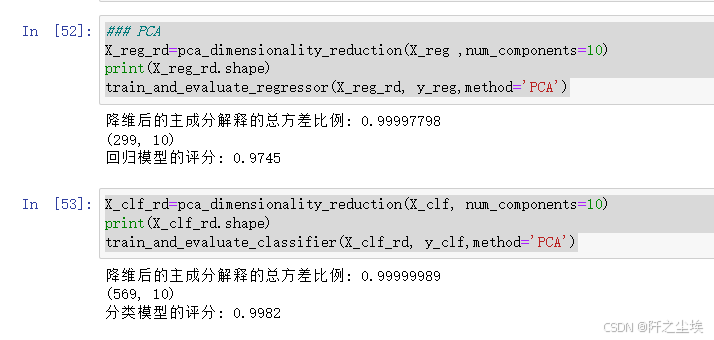

IPCA使用：

X_reg_rd=pca_dimensionality_reduction(X_reg ,num_components=10)
print(X_reg_rd.shape)
train_and_evaluate_regressor(X_reg_rd, y_reg,method='IPCA')
X_clf_rd=pca_dimensionality_reduction(X_clf, num_components=10)
print(X_clf_rd.shape)
train_and_evaluate_classifier(X_clf_rd, y_clf,method='IPCA')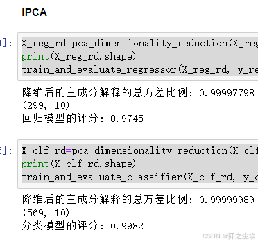

KPCA使用

X_reg_rd=pca_dimensionality_reduction(X_reg ,num_components=10)
print(X_reg_rd.shape)
train_and_evaluate_regressor(X_reg_rd, y_reg,method='KPCA')
X_clf_rd=pca_dimensionality_reduction(X_clf, num_components=10)
print(X_clf_rd.shape)
train_and_evaluate_classifier(X_clf_rd, y_clf,method='KPCA')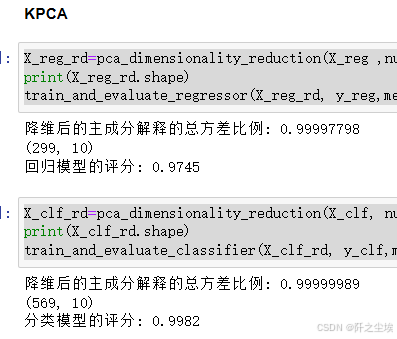

SparsePCA使用

X_reg_rd=pca_dimensionality_reduction(X_reg ,num_components=10)
print(X_reg_rd.shape)
train_and_evaluate_regressor(X_reg_rd, y_reg,method='SPCA')
X_clf_rd=pca_dimensionality_reduction(X_clf, num_components=10)
print(X_clf_rd.shape)
train_and_evaluate_classifier(X_clf_rd, y_clf,method='SPCA')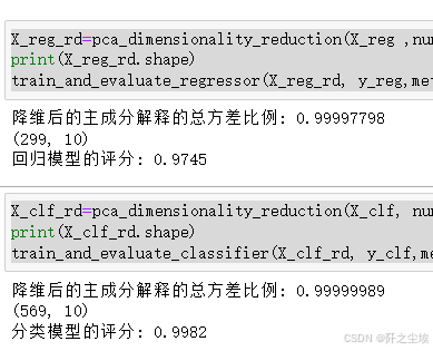

---

因子分析降维

和主成分是类似的

from sklearn.decomposition import FactorAnalysis
def factor_analysis_dimensionality_reduction(X, num_components=None):
    """
    使用因子分析（FA）进行降维。
    参数:
    - X: pandas DataFrame，包含原始特征。
    - num_components: int，选择的因子数量（如果为None，则保留所有因子）。
    返回:
    - pandas DataFrame，包含降维后的数据。
    """
    # 初始化因子分析模型
    fa = FactorAnalysis(n_components=num_components, random_state=0)
    
    # 拟合并转换数据
    X_fa = fa.fit_transform(X)
    
    # 为降维后的数据创建 DataFrame
    component_names = [f'Factor{i+1}' for i in range(X_fa.shape[1])]
    X_fa_df = pd.DataFrame(X_fa, columns=component_names)
    
    return X_fa_df

使用

X_reg_rd=factor_analysis_dimensionality_reduction(X_reg ,num_components=10)
print(X_reg_rd.shape)
train_and_evaluate_regressor(X_reg_rd, y_reg,method='FA')
X_clf_rd=factor_analysis_dimensionality_reduction(X_clf, num_components=10)
print(X_clf_rd.shape)
train_and_evaluate_classifier(X_clf_rd, y_clf,method='FA')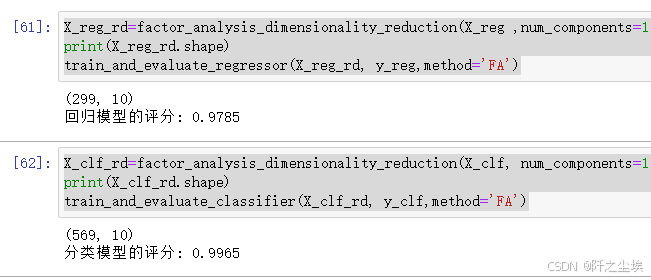

PLS偏最小二乘降维

from sklearn.cross_decomposition import PLSRegression
def pls_dimensionality_reduction(X, y, num_components=None):
    """
    使用偏最小二乘回归（PLS）进行降维。

    参数:
    - X: pandas DataFrame，包含原始特征。
    - y: pandas Series 或 DataFrame，目标变量。
    - num_components: int，选择的成分数量（如果为None，则默认使用所有成分）。

    返回:
    - pandas DataFrame，包含降维后的数据。
    """
    # 初始化 PLS 模型
    pls = PLSRegression(n_components=num_components)
    
    # 拟合模型并转换数据
    X_pls = pls.fit_transform(X, y)[0]
    
    # 为降维后的数据创建 DataFrame
    component_names = [f'PLS_Component{i+1}' for i in range(X_pls.shape[1])]
    X_pls_df = pd.DataFrame(X_pls, columns=component_names)
    
    return X_pls_df

使用

X_reg_rd=pls_dimensionality_reduction(X_reg ,y_reg,num_components=10)
print(X_reg_rd.shape)
train_and_evaluate_regressor(X_reg_rd, y_reg,method='PLS')
X_clf_rd=pls_dimensionality_reduction(X_clf, y_clf,num_components=10)
print(X_clf_rd.shape)
train_and_evaluate_classifier(X_clf_rd, y_clf,method='PLS')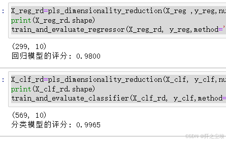

线性判别分析（LDA）

这个方法只能分类问题用。

from sklearn.discriminant_analysis import LinearDiscriminantAnalysis
import pandas as pd

def lda_dimensionality_reduction(X, y, num_components=None):
    """
    使用线性判别分析（LDA）进行降维。

    参数:
    - X: pandas DataFrame，包含原始特征。
    - y: pandas Series，目标类别标签。
    - num_components: int，选择的成分数量（如果为None，则使用最大可能的成分数）。

    返回:
    - pandas DataFrame，包含降维后的数据。
    """
    # 初始化 LDA 模型
    lda = LinearDiscriminantAnalysis(n_components=num_components)
    
    # 拟合模型并转换数据
    X_lda = lda.fit_transform(X, y)
    
    # 为降维后的数据创建 DataFrame
    component_names = [f'LDA_Component{i+1}' for i in range(X_lda.shape[1])]
    X_lda_df = pd.DataFrame(X_lda, columns=component_names)
    
    return X_lda_df

使用、

X_clf_rd=lda_dimensionality_reduction(X_clf, y_clf,num_components=1)
print(X_clf_rd.shape)
train_and_evaluate_classifier(X_clf_rd, y_clf,method='LDA')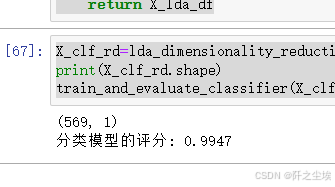

---

奇异值分解SVD降维

from sklearn.decomposition import TruncatedSVD
from scipy.linalg import svd as scipy_svd  # 避免与变量名冲突

def svd_based_dimensionality_reduction(X, method='SVD', num_components=None):
    """
    使用指定的 SVD 基方法进行降维。

    参数:
    - X: pandas DataFrame，包含原始特征。
    - method: str，选择降维方法，'SVD' 或 'TruncatedSVD'。
    - num_components: int，选择的成分数量（如果为 None，则使用所有成分）。

    返回:
    - pandas DataFrame，包含降维后的数据。
    """
    if num_components is None or num_components > min(X.shape):
        num_components = min(X.shape) - 1  # 防止选择超过可能的最大成分数

    if method == 'SVD':
        # 使用标准 SVD
        U, Sigma, VT = scipy_svd(X, full_matrices=False)
        X_reduced = U[:, :num_components] @ np.diag(Sigma[:num_components])

    elif method == 'TruncatedSVD':
        # 使用截断的 SVD (LSA)
        svd = TruncatedSVD(n_components=num_components, random_state=0)
        X_reduced = svd.fit_transform(X)

    else:
        raise ValueError("method 参数必须是 'SVD' 或 'TruncatedSVD'。")

    # 为降维后的数据创建 DataFrame
    component_names = [f'Component_{i+1}' for i in range(X_reduced.shape[1])]
    X_reduced_df = pd.DataFrame(X_reduced, columns=component_names)
    
    return X_reduced_df

SVD使用

X_reg_rd=svd_based_dimensionality_reduction(X_reg ,num_components=10, method='SVD')
print(X_reg_rd.shape)
train_and_evaluate_regressor(X_reg_rd, y_reg,method='SVD')
X_clf_rd=svd_based_dimensionality_reduction(X_clf,num_components=10, method='SVD')
print(X_clf_rd.shape)
train_and_evaluate_classifier(X_clf_rd, y_clf,method='SVD')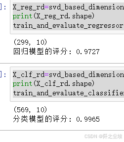

截断SVD（TruncatedSVD）

X_reg_rd=svd_based_dimensionality_reduction(X_reg ,num_components=10, method='TruncatedSVD')
print(X_reg_rd.shape)
train_and_evaluate_regressor(X_reg_rd, y_reg,method='TruncatedSVD')
X_clf_rd=svd_based_dimensionality_reduction(X_clf,num_components=10, method='TruncatedSVD')
print(X_clf_rd.shape)
train_and_evaluate_classifier(X_clf_rd, y_clf,method='TruncatedSVD')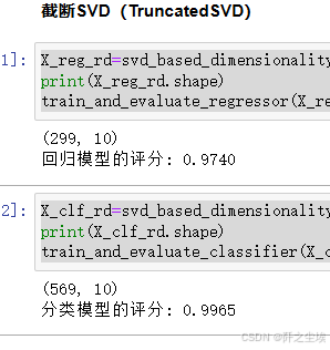

---

非负矩阵分解（NMF）

from sklearn.decomposition import NMF

def nmf_dimensionality_reduction(X, num_components=None):
    """
    使用非负矩阵分解（NMF）进行降维。

    参数:
    - X: pandas DataFrame，包含原始特征，要求所有元素为非负。
    - num_components: int，选择的成分数量（如果为 None，则使用所有特征数减一）。

    返回:
    - pandas DataFrame，包含降维后的数据。
    """
    if num_components is None or num_components > X.shape[1]:
        num_components = min(X.shape) - 1  # 防止选择超过可能的最大成分数

    # 初始化 NMF 模型
    nmf = NMF(n_components=num_components, random_state=0)
    
    # 拟合并转换数据
    X_nmf = nmf.fit_transform(np.abs(X))
    
    # 为降维后的数据创建 DataFrame
    component_names = [f'NMF_Component_{i+1}' for i in range(X_nmf.shape[1])]
    X_nmf_df = pd.DataFrame(X_nmf, columns=component_names)
    
    return X_nmf_df

使用

X_reg_rd=nmf_dimensionality_reduction(X_reg ,num_components=10)
print(X_reg_rd.shape)
train_and_evaluate_regressor(X_reg_rd, y_reg,method='NMF')
X_clf_rd=nmf_dimensionality_reduction(X_clf,num_components=10)
print(X_clf_rd.shape)
train_and_evaluate_classifier(X_clf_rd, y_clf,method='NMF')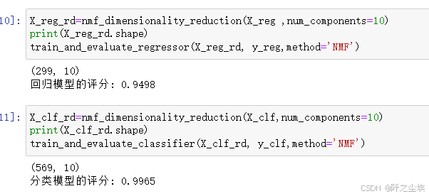

---

 

独立成分分析（ICA）

from sklearn.decomposition import FastICA

def ica_dimensionality_reduction(X, num_components=None):
    """
    使用独立成分分析（ICA）进行降维。

    参数:
    - X: pandas DataFrame，包含原始特征。
    - num_components: int，选择的成分数量（如果为 None，则使用所有特征数）。

    返回:
    - pandas DataFrame，包含降维后的数据。
    """
    if num_components is None or num_components > X.shape[1]:
        num_components = X.shape[1]  # 防止选择超过可能的最大成分数

    # 初始化 ICA 模型
    ica = FastICA(n_components=num_components, random_state=0)
    
    # 拟合并转换数据
    X_ica = ica.fit_transform(X)
    
    # 为降维后的数据创建 DataFrame
    component_names = [f'ICA_Component_{i+1}' for i in range(X_ica.shape[1])]
    X_ica_df = pd.DataFrame(X_ica, columns=component_names)
    
    return X_ica_df

使用

X_reg_rd=ica_dimensionality_reduction(X_reg ,num_components=10)
print(X_reg_rd.shape)
train_and_evaluate_regressor(X_reg_rd, y_reg,method='ICA')
X_clf_rd=ica_dimensionality_reduction(X_clf,num_components=10)
print(X_clf_rd.shape)
train_and_evaluate_classifier(X_clf_rd, y_clf,method='ICA')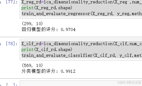

---

上面这些线性特征的方法都是类似的接口，函数写得都差不多，下面的非线性也差不多。

非线性特征提取

局部线性嵌入（Locally Linear Embedding, LLE）

from sklearn.manifold import LocallyLinearEmbedding

def lle_dimensionality_reduction(X, num_components=None, n_neighbors=10):
    """
    使用局部线性嵌入（LLE）进行降维。

    参数:
    - X: pandas DataFrame，包含原始特征。
    - num_components: int，选择的成分数量（如果为 None，则使用所有特征数减一）。
    - n_neighbors: int，选择用于 LLE 的邻居数量。

    返回:
    - pandas DataFrame，包含降维后的数据。
    """
    if num_components is None or num_components > X.shape[1]:
        num_components = min(X.shape) - 1  # 防止选择超过可能的最大成分数
    # 初始化 LLE 模型
    lle = LocallyLinearEmbedding(n_components=num_components, n_neighbors=n_neighbors)
    # 拟合并转换数据
    X_lle = lle.fit_transform(X)
    
    # 为降维后的数据创建 DataFrame
    component_names = [f'LLE_Component_{i+1}' for i in range(X_lle.shape[1])]
    X_lle_df = pd.DataFrame(X_lle, columns=component_names)
    return X_lle_df

使用

X_reg_rd=lle_dimensionality_reduction(X_reg ,num_components=10)
print(X_reg_rd.shape)
train_and_evaluate_regressor(X_reg_rd, y_reg,method='LLE')
X_clf_rd=lle_dimensionality_reduction(X_clf,num_components=10)
print(X_clf_rd.shape)
train_and_evaluate_classifier(X_clf_rd, y_clf,method='LLE')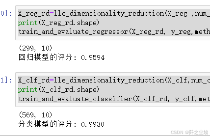

---

拉普拉斯特征映射（Laplacian Eigenmaps）

from sklearn.manifold import SpectralEmbedding
import pandas as pd

def le_dimensionality_reduction(X, num_components=None, n_neighbors=10):
    """
    使用拉普拉斯特征映射（Laplacian Eigenmaps）进行降维。

    参数:
    - X: pandas DataFrame，包含原始特征。
    - num_components: int，选择的成分数量（如果为 None，则使用所有特征数减一）。
    - n_neighbors: int，选择用于构建图的邻居数量。

    返回:
    - pandas DataFrame，包含降维后的数据。
    """
    if num_components is None or num_components > X.shape[1]:
        num_components = min(X.shape) - 1  # 防止选择超过可能的最大成分数

    # 初始化 Spectral Embedding 模型
    le = SpectralEmbedding(n_components=num_components, n_neighbors=n_neighbors)
    # 拟合并转换数据
    X_le = le.fit_transform(X)
    
    # 为降维后的数据创建 DataFrame
    component_names = [f'LE_Component_{i+1}' for i in range(X_le.shape[1])]
    X_le_df = pd.DataFrame(X_le, columns=component_names)
    return X_le_df

使用

X_reg_rd=le_dimensionality_reduction(X_reg ,num_components=10)
print(X_reg_rd.shape)
train_and_evaluate_regressor(X_reg_rd, y_reg,method='LE')
X_clf_rd=le_dimensionality_reduction(X_clf,num_components=10)
print(X_clf_rd.shape)
train_and_evaluate_classifier(X_clf_rd, y_clf,method='LE')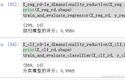

多维尺度分析（Multidimensional Scaling, MDS）

from sklearn.manifold import MDS
import pandas as pd

def mds_dimensionality_reduction(X, num_components=2):
    """
    使用多维尺度分析（MDS）进行降维。

    参数:
    - X: pandas DataFrame，包含原始特征。
    - num_components: int，选择的成分数量（通常为2，用于可视化）。

    返回:
    - pandas DataFrame，包含降维后的数据。
    """
    # 初始化 MDS 模型
    mds = MDS(n_components=num_components, random_state=0)
    
    # 拟合并转换数据
    X_mds = mds.fit_transform(X)
    
    # 为降维后的数据创建 DataFrame
    component_names = [f'MDS_Component_{i+1}' for i in range(X_mds.shape[1])]
    X_mds_df = pd.DataFrame(X_mds, columns=component_names)
    
    return X_mds_df

使用

X_reg_rd=mds_dimensionality_reduction(X_reg ,num_components=3)
print(X_reg_rd.shape)
train_and_evaluate_regressor(X_reg_rd, y_reg,method='MDS')
X_clf_rd=mds_dimensionality_reduction(X_clf,num_components=3)
print(X_clf_rd.shape)
train_and_evaluate_classifier(X_clf_rd, y_clf,method='MDS')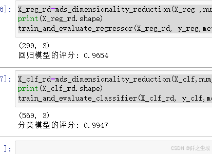

t-SNE（t-Distributed Stochastic Neighbor Embedding）

from sklearn.manifold import TSNE
def tsne_dimensionality_reduction(X, num_components=2, perplexity=30.0, n_iter=1000):
    """
    使用 t-SNE 进行降维。

    参数:
    - X: pandas DataFrame，包含原始特征。
    - num_components: int，选择的成分数量（通常为2，用于可视化）。
    - perplexity: float，控制 t-SNE 中的近邻权重（通常在 5 到 50 之间）。
    - n_iter: int，优化的迭代次数。

    返回:
    - pandas DataFrame，包含降维后的数据。
    """
    # 初始化 t-SNE 模型
    tsne = TSNE(n_components=num_components, perplexity=perplexity, n_iter=n_iter, random_state=0)
    
    # 拟合并转换数据
    X_tsne = tsne.fit_transform(X)
    
    # 为降维后的数据创建 DataFrame
    component_names = [f'TSNE_Component_{i+1}' for i in range(X_tsne.shape[1])]
    X_tsne_df = pd.DataFrame(X_tsne, columns=component_names)
    
    return X_tsne_df

使用

X_reg_rd=mds_dimensionality_reduction(X_reg ,num_components=3)
print(X_reg_rd.shape)
train_and_evaluate_regressor(X_reg_rd, y_reg,method='T-sne')
X_clf_rd=mds_dimensionality_reduction(X_clf,num_components=3)
print(X_clf_rd.shape)
train_and_evaluate_classifier(X_clf_rd, y_clf,method='T-sne')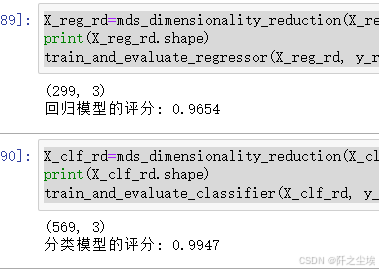

Isomap

from sklearn.manifold import Isomap
def isomap_dimensionality_reduction(X, num_components=2, n_neighbors=5):
    """
    使用 Isomap 进行降维。

    参数:
    - X: pandas DataFrame，包含原始特征。
    - num_components: int，选择的成分数量。
    - n_neighbors: int，构建图时使用的邻居数量。

    返回:
    - pandas DataFrame，包含降维后的数据。
    """
    # 初始化 Isomap 模型
    isomap = Isomap(n_components=num_components, n_neighbors=n_neighbors)
    
    # 拟合并转换数据
    X_isomap = isomap.fit_transform(X)
    
    # 为降维后的数据创建 DataFrame
    component_names = [f'Isomap_Component_{i+1}' for i in range(X_isomap.shape[1])]
    X_isomap_df = pd.DataFrame(X_isomap, columns=component_names)
    
    return X_isomap_df

使用

X_reg_rd=isomap_dimensionality_reduction(X_reg ,num_components=3)
print(X_reg_rd.shape)
train_and_evaluate_regressor(X_reg_rd, y_reg,method='ISOMAP')
X_clf_rd=isomap_dimensionality_reduction(X_clf,num_components=3)
print(X_clf_rd.shape)
train_and_evaluate_classifier(X_clf_rd, y_clf,method='ISOMAP')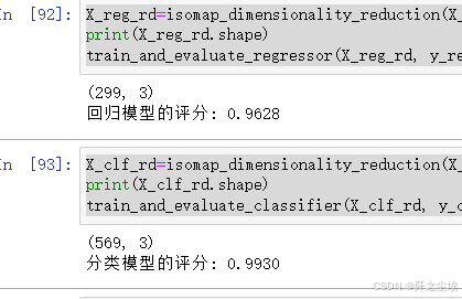

自编码器Autoencoders

# from tensorflow.keras.layers import Input, Dense
# from tensorflow.keras.models import Model
# from tensorflow.keras.optimizers import Adam

# def autoencoder_dimensionality_reduction(X, num_components=2, epochs=50, batch_size=32):
#     """
#     使用自编码器进行降维。
#     参数:
#     - X: numpy array 或 pandas DataFrame，包含原始特征。
#     - num_components: int，选择的成分数量（编码层的维度）。
#     - epochs: int，训练的轮数。
#     - batch_size: int，训练时的批次大小。

#     返回:
#     - pandas DataFrame，包含降维后的数据。
#     """
#     # 确保输入数据是 numpy array
#     if isinstance(X, pd.DataFrame):
#         X = X.to_numpy()

#     # 输入的维度
#     input_dim = X.shape[1]

#     # 定义自编码器模型
#     input_layer = Input(shape=(input_dim,))
#     # 编码层
#     encoded = Dense(num_components, activation='relu')(input_layer)
#     # 解码层
#     decoded = Dense(input_dim, activation='sigmoid')(encoded)

#     # 构建自编码器模型
#     autoencoder = Model(inputs=input_layer, outputs=decoded)

#     # 编译自编码器
#     autoencoder.compile(optimizer=Adam(), loss='mean_squared_error')

#     # 训练自编码器
#     autoencoder.fit(X, X, epochs=epochs, batch_size=batch_size, shuffle=True, verbose=1)

#     # 提取编码器模型
#     encoder = Model(inputs=input_layer, outputs=encoded)

#     # 将数据通过编码器进行降维
#     X_encoded = encoder.predict(X)

#     # 为降维后的数据创建 DataFrame
#     component_names = [f'AE_Component_{i+1}' for i in range(X_encoded.shape[1])]
#     X_encoded_df = pd.DataFrame(X_encoded, columns=component_names)

#     return X_encoded_df

使用

# X_reg_rd=autoencoder_dimensionality_reduction(X_reg ,num_components=10)
# print(X_reg_rd.shape)
# train_and_evaluate_regressor(X_reg_rd, y_reg,method='AE')
# X_clf_rd=autoencoder_dimensionality_reduction(X_clf,num_components=10)
# print(X_clf_rd.shape)
# train_and_evaluate_classifier(X_clf_rd, y_clf,method='AE')

由于这个代码需要keras库，我写代码的这个环境没装，就不运行了。

---

结果可视化对比

对不同方法的准确率进行可视化

# 创建1x2的子图
fig, axes = plt.subplots(2, 1, figsize=(12, 5),dpi=128)

# 绘制分类模型的柱状图
axes[0].bar(df_eval_clf.index, df_eval_clf['score'], color='skyblue')
axes[0].set_title('Classification Model Accuracy')
axes[0].set_ylim(0.95, 1.0)  # 设置基准轴起始位置
axes[0].set_ylabel('Accuracy')
axes[0].set_xticklabels(df_eval_clf.index, rotation=45) 

# 绘制回归模型的柱状图
axes[1].bar(df_eval_reg.index, df_eval_reg['score'], color='salmon')
axes[1].set_title('Regression Model R2 Score')
axes[1].set_ylim(0.95, 1.0)  # 设置基准轴起始位置
axes[1].set_ylabel('R2 Score')
axes[1].set_xticklabels(df_eval_clf.index, rotation=45) 

# 调整子图布局
plt.tight_layout()

# 显示图形
plt.show()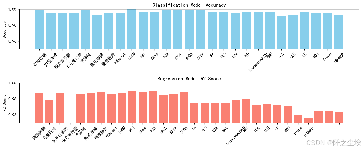

从分类问题来看，这个数据集上，LGBM的模型姜维效果似乎是最好的，其他模型降维效果差不多。

回归问题来看，PCA和SPCA比较好，其他线性和非线性效果一般。

---

总结

其实没有最好的方法，对于不同的数据要采用不同的方法尝试。

本文也不讲原理，基本上所有的降维方法都进行抽象函数化，接口和使用方法统一，主要是方便使用，实用为主，全面总结，应该没有别的更多的常见的降维方法了。

以前的文章可以参考：实用的Python机器学习_阡之尘埃的博客

数据分析案例可以参考：Python数据分析案例_阡之尘埃的博客

创作不易，看官觉得写得还不错的话点个关注和赞吧，本人会持续更新python数据分析领域的代码文章~(需要定制类似的代码可私信)