


吴恩达课后编程作业:改善神经网络
1、分割数据集:
1.1导包:
import numpy as np
import matplotlib.pyplot as plt
import scipy.io
import math
import sklearn
import sklearn.datasets

import opt_utils #参见数据包或者在本文底部copy
import testCase  #参见数据包或者在本文底部copy

#%matplotlib inline #如果你用的是Jupyter Notebook请取消注释
plt.rcParams['figure.figsize'] = (7.0, 4.0) # set default size of plots
plt.rcParams['image.interpolation'] = 'nearest'
plt.rcParams['image.cmap'] = 'gray'
2、优化梯度下降算法:
为什么要使用优化梯度下降算法呢?
答:能够在一定程度上加快了算法的收敛程序,能够更好更快地分离结果,加快学习速度。例如,下山的时候,每次都往下走(有多个方向),优化梯度下降就是为了找到一条尽可能好的路径,达到山脚,若只是单纯地使用标准的梯度下降算法的话,可能向左右走的幅度非常大,而向下走的幅度比较小,所以你会通过优化算法,减少左右移动的幅度,而增大向下走的幅度。
2.1、不使用任何优化算法
2.1.1. 标准梯度下降算法
def update_parameters_with_gd(parameters,grads,learning_rate):
    L = len(parameters)//2 #因为parameters中保存了W和b两个
    for l in range(L):
        parameters["W"+str(l +1)] =  parameters["W"+str(l+1)] - learning_rate * grads["dW"+str(l+1)]
        parameters["b"+str(l +1)] =  parameters["b"+str(l+1)] - learning_rate * grads["db"+str(l+1)]
    return parameters
2.1.2 测试:
#测试update_parameters_with_gd
print("-------------测试update_parameters_with_gd-------------")
parameters , grads , learning_rate = testCase.update_parameters_with_gd_test_case()
parameters = update_parameters_with_gd(parameters,grads,learning_rate)
print("W1 = " + str(parameters["W1"]))
print("b1 = " + str(parameters["b1"]))
print("W2 = " + str(parameters["W2"]))
print("b2 = " + str(parameters["b2"]))
2.2、 mini_batch 梯度下降算法
2.2.1 进行数据的分割
def random_mini_batches (X,Y,mini_batch_size=64,seed=0):
    np.random.seed(seed)
    m = X.shape[1]
    mini_batches = []
    #打乱顺序
    permutation = list(np.random.permutation(m)) #返回一个长度为m 的随机数组
    shuffled_X = X[:,permutation]
    shuffled_Y = Y[:,permutation].reshape((1,m))

    #分割
    num_complete_minibatches = math.floor(m / mini_batch_size)  #将被分割成多少分
    for k in range(0,num_complete_minibatches):
        # : 表示选择所有行,k * mini_batch_size 表示起始下标,(k+1) * mini_batch_size 表示终止下标
        mini_batch_X = shuffled_X[:,k * mini_batch_size:(k+1) *mini_batch_size]
        mini_batch_Y = shuffled_Y[:,k * mini_batch_size:(k+1) *mini_batch_size]
        mini_batch = (mini_batch_X,mini_batch_Y)
        mini_batches.append(mini_batch)
    if  m % mini_batch_size != 0:
     # 因为若训练集不是64的整数倍的话,则必定有剩余部分,进行处理
     mini_batch_X = shuffled_X[:, mini_batch_size * num_complete_minibatches:]
     mini_batch_Y = shuffled_Y[:, mini_batch_size * num_complete_minibatches:]
     mini_batch = (mini_batch_X, mini_batch_Y)
     mini_batches.append(mini_batch)

     return mini_batches
2.2.2. 运行测试:
#测试random_mini_batches
print("-------------测试random_mini_batches-------------")
X_assess,Y_assess,mini_batch_size = testCase.random_mini_batches_test_case()
mini_batches = random_mini_batches(X_assess,Y_assess,mini_batch_size)

print("第1个mini_batch_X 的维度为:",mini_batches[0][0].shape)
print("第1个mini_batch_Y 的维度为:",mini_batches[0][1].shape)
print("第2个mini_batch_X 的维度为:",mini_batches[1][0].shape)
print("第2个mini_batch_Y 的维度为:",mini_batches[1][1].shape)
print("第3个mini_batch_X 的维度为:",mini_batches[2][0].shape)
print("第3个mini_batch_Y 的维度为:",mini_batches[2][1].shape)
对比mini_batch梯度算法 和随机梯度算法:
mini_batch梯度算法:是将训练集分割成为一个大小为m (1<m<训练集集)的子集合,也称为小批量梯度下降算法,对m个样本同时进行训练,m的大小一般为2的n次方,充分使用了GPU的并行性,相比于随机梯度算法,能够更加平稳地收敛,且波动不大。
随机梯度算法:每次只选择一个样本进行驯良,运行速度很快,但是波动也大,不会平稳地收敛。
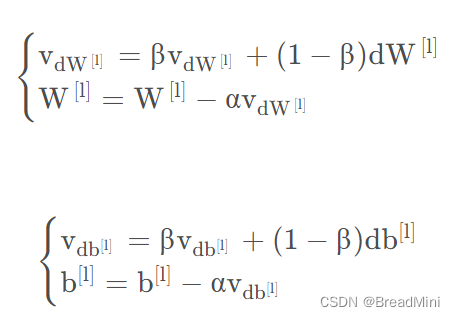
2.3、moment动量梯度下降算法
由于minI_batch梯度下降算法每次只能看到一个子集合的参数更新,所以可能造成该算法是大幅度振荡走向收敛的(也就是下山不是直直到达山脚的,乱走),使用动量可以减少这些振荡,因为动量考虑了以前的梯度,不只是考虑当前的梯度,将其数据存储在变量v中,也就是指数加权平均数了,越是距离当前位置远的梯度呢,影响就会越小。可以由公式知道,V dW =β⋅VdW +(1−β)⋅dW。
2.3.1 初始化v矩阵
def initialize_velocity(parameters):
    L = len(parameters)//2
    v = {}
    for l in range(L):
        #生成与权重W,和偏置b相同矩阵格式的dw,db的零矩阵
        v["dW" + str(l + 1)] = np.zeros_like(parameters["W" + str(l+1)])
        v["db" + str(l + 1)] = np.zeros_like(parameters["b" + str(l+1)])
    return v
2.3.2 运行测试
#测试initialize_velocity
print("-------------测试initialize_velocity-------------")
parameters = testCase.initialize_velocity_test_case()
v = initialize_velocity(parameters)

print('v["dW1"] = ' + str(v["dW1"]))
print('v["db1"] = ' + str(v["db1"]))
print('v["dW2"] = ' + str(v["dW2"]))
print('v["db2"] = ' + str(v["db2"]))
2.3.3 计算并更新参数
def update_parameters_with_momentun(parameters,grads,v,beta,learning_rate):
    """

    :param parameters:
    :param grads:
    :param v:
    v - 一个字典变量,包含了以下参数:
     v["dW" + str(l)] = dWl的速度
     v["db" + str(l)] = dbl的速度
    :param beta: 超参数,动量,实数
    :param learning_rate:
    :return:
    """
    L = len(parameters)//2
    for l in range(L):
        #计算指数加权平均值
        v["dW" + str(l+1)] = beta * v["dW" + str(l+1)] + (1 - beta) * grads["dW" + str(l+1)]
        v["db" + str(l+1)] = beta * v["db" + str(l+1)] + (1 - beta) * grads["db" + str(l+1)]
        #更新参数
        parameters["W" + str(l+1)] =  parameters["W" + str(l+1)] - learning_rate *  v["dW" + str(l+1)]
        parameters["b" + str(l+1)] =  parameters["b" + str(l+1)] - learning_rate *  v["db" + str(l+1)]
    return parameters,v
2.3.4 运行测试:
#测试update_parameters_with_momentun
print("-------------测试update_parameters_with_momentun-------------")
parameters,grads,v = testCase.update_parameters_with_momentum_test_case()
update_parameters_with_momentun(parameters,grads,v,beta=0.9,learning_rate=0.01)

print("W1 = " + str(parameters["W1"]))
print("b1 = " + str(parameters["b1"]))
print("W2 = " + str(parameters["W2"]))
print("b2 = " + str(parameters["b2"]))
print('v["dW1"] = ' + str(v["dW1"]))
print('v["db1"] = ' + str(v["db1"]))
print('v["dW2"] = ' + str(v["dW2"]))
print('v["db2"] = ' + str(v["db2"]))
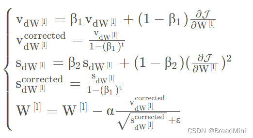
2.4、Adam算法
Adam算法是综合Moment 动量梯度下降算法和mini_batch 梯度下降算法,以达到更好的效果,事实证明,该算法能够广泛应用在神经网络中。
2.4.1 所用到的公式:
2.4.2 初始化存储矩阵:
def initialize_adam(parameters):
    L = len(parameters)//2
    v = {}
    s = {}
    for l in range(L):
        v["dW" + str(l + 1)] = np.zeros_like(parameters["W" + str(l + 1)])
        v["db" + str(l + 1)] = np.zeros_like(parameters["b" + str(l + 1)])
        s["dW" + str(l + 1)] = np.zeros_like(parameters["W" + str(l + 1)])
        s["db" + str(l + 1)] = np.zeros_like(parameters["b" + str(l + 1)])
    return (v,s)
2.4.3 更新参数:
def update_parameters_with_adam(parameters,grads,v,s,t,learning_rate=0.01,beta1=0.9,beta2=0.999,epsilon=1e-8):
    L = len(parameters)//2
    v_corrected = {}    #偏差修正后的值
    s_corrected = {}    #偏差修正后的值
    for l in range(L):
        v["dW" + str(l + 1)] = beta1 * v["dW" + str(l + 1)] + (1 - beta1) * grads["dW" + str(l + 1)]
        v["db" + str(l + 1)] = beta1 * v["db" + str(l + 1)] + (1 - beta1) * grads["db" + str(l + 1)]
        #计算偏差修正后的估计值
        v_corrected["dW" + str(l + 1)] = v["dW" + str(l + 1)] /(1 - np.power(beta1,t))
        v_corrected["db" + str(l + 1)] = v["db" + str(l + 1)] /(1 - np.power(beta1,t))
        s["dW" + str(l + 1)] = beta2 * s["dW" + str(l + 1)] + (1 - beta2) * (np.square(grads["dW" + str(l + 1)]))
        s["db" + str(l + 1)] = beta2 * s["db" + str(l + 1)] +  (1 - beta2) * (np.square(grads["db" + str(l + 1)]))
        # 计算偏差修正后的估计值
        s_corrected["dW" + str(l + 1)] = s["dW" + str(l + 1)] / (1 - np.power(beta2, t))
        s_corrected["db" + str(l + 1)] = s["db" + str(l + 1)] / (1 - np.power(beta2, t))
        #更新参数
        parameters["W" + str(l+1)] =  parameters["W" + str(l+1)] - learning_rate * (v_corrected["dW" + str(l + 1)]/(np.sqrt(s_corrected["dW" + str(l + 1)])+epsilon))
        parameters["b" + str(l+1)] =  parameters["b" + str(l+1)] - learning_rate * (v_corrected["db" + str(l + 1)]/(np.sqrt(s_corrected["db" + str(l + 1)])+epsilon))
    return (parameters,v,s)

train_X,train_Y  = opt_utils.load_dataset(is_plot=True)
3、整合模型
def model(X, Y, layers_dims, optimizer, learning_rate=0.0007,
          mini_batch_size=64, beta=0.9, beta1=0.9, beta2=0.999,
          epsilon=1e-8, num_epochs=10000, print_cost=True, is_plot=True):
    """
    可以运行在不同优化器模式下的3层神经网络模型。

    参数:
        X - 输入数据,维度为(2,输入的数据集里面样本数量)
        Y - 与X对应的标签
        layers_dims - 包含层数和节点数量的列表
        optimizer - 字符串类型的参数,用于选择优化类型,【 "gd" | "momentum" | "adam" 】
        learning_rate - 学习率
        mini_batch_size - 每个小批量数据集的大小
        beta - 用于动量优化的一个超参数
        beta1 - 用于计算梯度后的指数衰减的估计的超参数
        beta1 - 用于计算平方梯度后的指数衰减的估计的超参数
        epsilon - 用于在Adam中避免除零操作的超参数,一般不更改
        num_epochs - 整个训练集的遍历次数,(视频2.9学习率衰减,1分55秒处,视频中称作“代”),相当于之前的num_iteration
        print_cost - 是否打印误差值,每遍历1000次数据集打印一次,但是每100次记录一个误差值,又称每1000代打印一次
        is_plot - 是否绘制出曲线图

    返回:
        parameters - 包含了学习后的参数

    """
    L = len(layers_dims)
    costs = []
    t = 0  # 每学习完一个minibatch就增加1
    seed = 10  # 随机种子

    # 初始化参数
    parameters = opt_utils.initialize_parameters(layers_dims)

    # 选择优化器
    if optimizer == "gd":
        pass  # 不使用任何优化器,直接使用梯度下降法
    elif optimizer == "momentum":
        v = initialize_velocity(parameters)  # 使用动量
    elif optimizer == "adam":
        v, s = initialize_adam(parameters)  # 使用Adam优化
    else:
        print("optimizer参数错误,程序退出。")
        exit(1)

    # 开始学习
    for i in range(num_epochs):
        # 定义随机 minibatches,我们在每次遍历数据集之后增加种子以重新排列数据集,使每次数据的顺序都不同
        seed = seed + 1
        minibatches = random_mini_batches(X, Y, mini_batch_size, seed)

        for minibatch in minibatches:
            # 选择一个minibatch
            (minibatch_X, minibatch_Y) = minibatch

            # 前向传播
            A3, cache = opt_utils.forward_propagation(minibatch_X, parameters)

            # 计算误差
            cost = opt_utils.compute_cost(A3, minibatch_Y)

            # 反向传播
            grads = opt_utils.backward_propagation(minibatch_X, minibatch_Y, cache)

            # 更新参数
            if optimizer == "gd":
                parameters = update_parameters_with_gd(parameters, grads, learning_rate)
            elif optimizer == "momentum":
                parameters, v = update_parameters_with_momentun(parameters, grads, v, beta, learning_rate)
            elif optimizer == "adam":
                t = t + 1
                parameters, v, s = update_parameters_with_adam(parameters, grads, v, s, t, learning_rate, beta1, beta2,
                                                               epsilon)
        # 记录误差值
        if i % 100 == 0:
            costs.append(cost)
            # 是否打印误差值
            if print_cost and i % 1000 == 0:
                print("第" + str(i) + "次遍历整个数据集,当前误差值:" + str(cost))
    # 是否绘制曲线图
    if is_plot:
        plt.plot(costs)
        plt.ylabel('cost')
        plt.xlabel('epochs (per 100)')
        plt.title("Learning rate = " + str(learning_rate))
        plt.show()

    return parameters
运行测试
#optimizer中选择不同的算法即可
layers_dims = [train_X.shape[0],5,2,1]
parameters = model(train_X, train_Y, layers_dims, optimizer="adam",is_plot=True)

#预测
preditions = opt_utils.predict(train_X,train_Y,parameters)

#绘制分类图
plt.title("Model with Gradient Descent optimization")
axes = plt.gca()
axes.set_xlim([-1.5, 2.5])
axes.set_ylim([-1, 1.5])
opt_utils.plot_decision_boundary(lambda x: opt_utils.predict_dec(parameters, x.T), train_X, train_Y)
4、工具类
opt_utils.py
# -*- coding: utf-8 -*-

#opt_utils.py

import numpy as np
import matplotlib.pyplot as plt
import sklearn
import sklearn.datasets

def sigmoid(x):
    """
    Compute the sigmoid of x

    Arguments:
    x -- A scalar or numpy array of any size.

    Return:
    s -- sigmoid(x)
    """
    s = 1/(1+np.exp(-x))
    return s

def relu(x):
    """
    Compute the relu of x

    Arguments:
    x -- A scalar or numpy array of any size.

    Return:
    s -- relu(x)
    """
    s = np.maximum(0,x)

    return s


def load_params_and_grads(seed=1):
    np.random.seed(seed)
    W1 = np.random.randn(2,3)
    b1 = np.random.randn(2,1)
    W2 = np.random.randn(3,3)
    b2 = np.random.randn(3,1)

    dW1 = np.random.randn(2,3)
    db1 = np.random.randn(2,1)
    dW2 = np.random.randn(3,3)
    db2 = np.random.randn(3,1)

    return W1, b1, W2, b2, dW1, db1, dW2, db2

def initialize_parameters(layer_dims):
    """
    Arguments:
    layer_dims -- python array (list) containing the dimensions of each layer in our network

    Returns:
    parameters -- python dictionary containing your parameters "W1", "b1", ..., "WL", "bL":
                    W1 -- weight matrix of shape (layer_dims[l], layer_dims[l-1])
                    b1 -- bias vector of shape (layer_dims[l], 1)
                    Wl -- weight matrix of shape (layer_dims[l-1], layer_dims[l])
                    bl -- bias vector of shape (1, layer_dims[l])

    Tips:
    - For example: the layer_dims for the "Planar Data classification model" would have been [2,2,1].
    This means W1's shape was (2,2), b1 was (1,2), W2 was (2,1) and b2 was (1,1). Now you have to generalize it!
    - In the for loop, use parameters['W' + str(l)] to access Wl, where l is the iterative integer.
    """

    np.random.seed(3)
    parameters = {}
    L = len(layer_dims) # number of layers in the network

    for l in range(1, L):
        parameters['W' + str(l)] = np.random.randn(layer_dims[l], layer_dims[l-1])*  np.sqrt(2 / layer_dims[l-1])
        parameters['b' + str(l)] = np.zeros((layer_dims[l], 1))

        assert(parameters['W' + str(l)].shape == layer_dims[l], layer_dims[l-1])
        assert(parameters['W' + str(l)].shape == layer_dims[l], 1)

    return parameters

def forward_propagation(X, parameters):
    """
    Implements the forward propagation (and computes the loss) presented in Figure 2.

    Arguments:
    X -- input dataset, of shape (input size, number of examples)
    parameters -- python dictionary containing your parameters "W1", "b1", "W2", "b2", "W3", "b3":
                    W1 -- weight matrix of shape ()
                    b1 -- bias vector of shape ()
                    W2 -- weight matrix of shape ()
                    b2 -- bias vector of shape ()
                    W3 -- weight matrix of shape ()
                    b3 -- bias vector of shape ()

    Returns:
    loss -- the loss function (vanilla logistic loss)
    """

    # retrieve parameters
    W1 = parameters["W1"]
    b1 = parameters["b1"]
    W2 = parameters["W2"]
    b2 = parameters["b2"]
    W3 = parameters["W3"]
    b3 = parameters["b3"]

    # LINEAR -> RELU -> LINEAR -> RELU -> LINEAR -> SIGMOID
    z1 = np.dot(W1, X) + b1
    a1 = relu(z1)
    z2 = np.dot(W2, a1) + b2
    a2 = relu(z2)
    z3 = np.dot(W3, a2) + b3
    a3 = sigmoid(z3)

    cache = (z1, a1, W1, b1, z2, a2, W2, b2, z3, a3, W3, b3)

    return a3, cache

def backward_propagation(X, Y, cache):
    """
    Implement the backward propagation presented in figure 2.

    Arguments:
    X -- input dataset, of shape (input size, number of examples)
    Y -- true "label" vector (containing 0 if cat, 1 if non-cat)
    cache -- cache output from forward_propagation()

    Returns:
    gradients -- A dictionary with the gradients with respect to each parameter, activation and pre-activation variables
    """
    m = X.shape[1]
    (z1, a1, W1, b1, z2, a2, W2, b2, z3, a3, W3, b3) = cache

    dz3 = 1./m * (a3 - Y)
    dW3 = np.dot(dz3, a2.T)
    db3 = np.sum(dz3, axis=1, keepdims = True)

    da2 = np.dot(W3.T, dz3)
    dz2 = np.multiply(da2, np.int64(a2 > 0))
    dW2 = np.dot(dz2, a1.T)
    db2 = np.sum(dz2, axis=1, keepdims = True)

    da1 = np.dot(W2.T, dz2)
    dz1 = np.multiply(da1, np.int64(a1 > 0))
    dW1 = np.dot(dz1, X.T)
    db1 = np.sum(dz1, axis=1, keepdims = True)

    gradients = {"dz3": dz3, "dW3": dW3, "db3": db3,
                 "da2": da2, "dz2": dz2, "dW2": dW2, "db2": db2,
                 "da1": da1, "dz1": dz1, "dW1": dW1, "db1": db1}

    return gradients

def compute_cost(a3, Y):

    """
    Implement the cost function

    Arguments:
    a3 -- post-activation, output of forward propagation
    Y -- "true" labels vector, same shape as a3

    Returns:
    cost - value of the cost function
    """
    m = Y.shape[1]

    logprobs = np.multiply(-np.log(a3),Y) + np.multiply(-np.log(1 - a3), 1 - Y)
    cost = 1./m * np.sum(logprobs)

    return cost

def predict(X, y, parameters):
    """
    This function is used to predict the results of a  n-layer neural network.

    Arguments:
    X -- data set of examples you would like to label
    parameters -- parameters of the trained model

    Returns:
    p -- predictions for the given dataset X
    """

    m = X.shape[1]
    p = np.zeros((1,m), dtype = np.int)

    # Forward propagation
    a3, caches = forward_propagation(X, parameters)

    # convert probas to 0/1 predictions
    for i in range(0, a3.shape[1]):
        if a3[0,i] > 0.5:
            p[0,i] = 1
        else:
            p[0,i] = 0

    # print results

    #print ("predictions: " + str(p[0,:]))
    #print ("true labels: " + str(y[0,:]))
    print("Accuracy: "  + str(np.mean((p[0,:] == y[0,:]))))

    return p

def predict_dec(parameters, X):
    """
    Used for plotting decision boundary.

    Arguments:
    parameters -- python dictionary containing your parameters
    X -- input data of size (m, K)

    Returns
    predictions -- vector of predictions of our model (red: 0 / blue: 1)
    """

    # Predict using forward propagation and a classification threshold of 0.5
    a3, cache = forward_propagation(X, parameters)
    predictions = (a3 > 0.5)
    return predictions

def plot_decision_boundary(model, X, y):
    # Set min and max values and give it some padding
    x_min, x_max = X[0, :].min() - 1, X[0, :].max() + 1
    y_min, y_max = X[1, :].min() - 1, X[1, :].max() + 1
    h = 0.01
    # Generate a grid of points with distance h between them
    xx, yy = np.meshgrid(np.arange(x_min, x_max, h), np.arange(y_min, y_max, h))
    # Predict the function value for the whole grid
    Z = model(np.c_[xx.ravel(), yy.ravel()])
    Z = Z.reshape(xx.shape)
    # Plot the contour and training examples
    plt.contourf(xx, yy, Z, cmap=plt.cm.Spectral)
    plt.ylabel('x2')
    plt.xlabel('x1')
    plt.scatter(X[0, :], X[1, :], c=y, cmap=plt.cm.Spectral)
    plt.show()

def load_dataset(is_plot = True):
    np.random.seed(3)
    train_X, train_Y = sklearn.datasets.make_moons(n_samples=300, noise=.2) #300 #0.2
    # Visualize the data
    if is_plot:
        plt.scatter(train_X[:, 0], train_X[:, 1], c=train_Y, s=40, cmap=plt.cm.Spectral);
    train_X = train_X.T
    train_Y = train_Y.reshape((1, train_Y.shape[0]))

    return train_X, train_Y
testCase.py
# -*- coding: utf-8 -*-

#testCase.py

import numpy as np

def update_parameters_with_gd_test_case():
    np.random.seed(1)
    learning_rate = 0.01
    W1 = np.random.randn(2,3)
    b1 = np.random.randn(2,1)
    W2 = np.random.randn(3,3)
    b2 = np.random.randn(3,1)

    dW1 = np.random.randn(2,3)
    db1 = np.random.randn(2,1)
    dW2 = np.random.randn(3,3)
    db2 = np.random.randn(3,1)

    parameters = {"W1": W1, "b1": b1, "W2": W2, "b2": b2}
    grads = {"dW1": dW1, "db1": db1, "dW2": dW2, "db2": db2}

    return parameters, grads, learning_rate

"""
def update_parameters_with_sgd_checker(function, inputs, outputs):
    if function(inputs) == outputs:
        print("Correct")
    else:
        print("Incorrect")
"""

def random_mini_batches_test_case():
    np.random.seed(1)
    mini_batch_size = 64
    X = np.random.randn(12288, 148)
    Y = np.random.randn(1, 148) < 0.5
    return X, Y, mini_batch_size

def initialize_velocity_test_case():
    np.random.seed(1)
    W1 = np.random.randn(2,3)
    b1 = np.random.randn(2,1)
    W2 = np.random.randn(3,3)
    b2 = np.random.randn(3,1)
    parameters = {"W1": W1, "b1": b1, "W2": W2, "b2": b2}
    return parameters

def update_parameters_with_momentum_test_case():
    np.random.seed(1)
    W1 = np.random.randn(2,3)
    b1 = np.random.randn(2,1)
    W2 = np.random.randn(3,3)
    b2 = np.random.randn(3,1)

    dW1 = np.random.randn(2,3)
    db1 = np.random.randn(2,1)
    dW2 = np.random.randn(3,3)
    db2 = np.random.randn(3,1)
    parameters = {"W1": W1, "b1": b1, "W2": W2, "b2": b2}
    grads = {"dW1": dW1, "db1": db1, "dW2": dW2, "db2": db2}
    v = {'dW1': np.array([[ 0.,  0.,  0.],
        [ 0.,  0.,  0.]]), 'dW2': np.array([[ 0.,  0.,  0.],
        [ 0.,  0.,  0.],
        [ 0.,  0.,  0.]]), 'db1': np.array([[ 0.],
        [ 0.]]), 'db2': np.array([[ 0.],
        [ 0.],
        [ 0.]])}
    return parameters, grads, v

def initialize_adam_test_case():
    np.random.seed(1)
    W1 = np.random.randn(2,3)
    b1 = np.random.randn(2,1)
    W2 = np.random.randn(3,3)
    b2 = np.random.randn(3,1)
    parameters = {"W1": W1, "b1": b1, "W2": W2, "b2": b2}
    return parameters

def update_parameters_with_adam_test_case():
    np.random.seed(1)
    v, s = ({'dW1': np.array([[ 0.,  0.,  0.],
         [ 0.,  0.,  0.]]), 'dW2': np.array([[ 0.,  0.,  0.],
         [ 0.,  0.,  0.],
         [ 0.,  0.,  0.]]), 'db1': np.array([[ 0.],
         [ 0.]]), 'db2': np.array([[ 0.],
         [ 0.],
         [ 0.]])}, {'dW1': np.array([[ 0.,  0.,  0.],
         [ 0.,  0.,  0.]]), 'dW2': np.array([[ 0.,  0.,  0.],
         [ 0.,  0.,  0.],
         [ 0.,  0.,  0.]]), 'db1': np.array([[ 0.],
         [ 0.]]), 'db2': np.array([[ 0.],
         [ 0.],
         [ 0.]])})
    W1 = np.random.randn(2,3)
    b1 = np.random.randn(2,1)
    W2 = np.random.randn(3,3)
    b2 = np.random.randn(3,1)

    dW1 = np.random.randn(2,3)
    db1 = np.random.randn(2,1)
    dW2 = np.random.randn(3,3)
    db2 = np.random.randn(3,1)

    parameters = {"W1": W1, "b1": b1, "W2": W2, "b2": b2}
    grads = {"dW1": dW1, "db1": db1, "dW2": dW2, "db2": db2}

    return parameters, grads, v, s


 620
620


 被折叠的 条评论
为什么被折叠?
被折叠的 条评论
为什么被折叠?
 到【灌水乐园】发言


