365天深度学习训练营-第P8周：YOLOv5-C3模块实现

weixin_46559155

已于 2023-12-05 10:19:22 修改

阅读量2.1k

点赞数 38

文章标签： YOLO 深度学习人工智能 python pytorch 多分类

于 2023-12-05 10:18:04 首次发布

本文链接：https://blog.csdn.net/weixin_46559155/article/details/134799157

版权

>- **🍨 本文为[🔗365天深度学习训练营] 中的学习记录博客
>- **🍖 原作者：[K同学啊 | 接辅导、项目定制]

一、前期准备

1.设置GPU

import torch
import torch.nn as nn
import torchvision
import torchvision.transforms as transforms
import PIL,os,pathlib,warnings
warnings.filterwarnings('ignore')

device = torch.device("cuda"if torch.cuda.is_available() else 'cpu')
device

device(type='cuda')

2.导入数据

def LocalData(root):
    data_dir = pathlib.Path(root)
    data_path = list(data_dir.glob("*"))
    ClassNames = [str(path).split("//")[-1] for path in data_path]
    
    train_transforms = transforms.Compose([
        transforms.Resize([224, 224]),
        transforms.ToTensor(),
        transforms.Normalize(
        mean=[0.486, 0.456, 0.406],
        std=[0.229, 0.224, 0.225])
    ])
    
    total_dataset = torchvision.datasets.ImageFolder(data_dir,transform=train_transforms)
    print(total_dataset)
    print(total_dataset.class_to_idx)
    
    train_size = int(0.8*len(total_dataset))
    test_size  = len(total_dataset)-train_size
    print('train_size:',train_size,'test_size:',test_size)
    
    train_dataset, test_dataset = torch.utils.data.random_split(total_dataset,[train_size,test_size])
    
    return ClassNames,train_dataset,test_dataset 

root = r'F:\Netural_work_Data\P3_data'
output = r'F:\model_param\p_8_model'
ClassNames ,train_dataset, test_dataset = LocalData(root)
print("图片类别数：",len(ClassNames))

Dataset ImageFolder
    Number of datapoints: 1125
    Root location: F:\Netural_work_Data\P3_data
    StandardTransform
Transform: Compose(
               Resize(size=[224, 224], interpolation=bilinear, max_size=None, antialias=warn)
               ToTensor()
               Normalize(mean=[0.486, 0.456, 0.406], std=[0.229, 0.224, 0.225])
           )
{'cloudy': 0, 'rain': 1, 'shine': 2, 'sunrise': 3}
train_size: 900 test_size: 225
图片类别数： 4

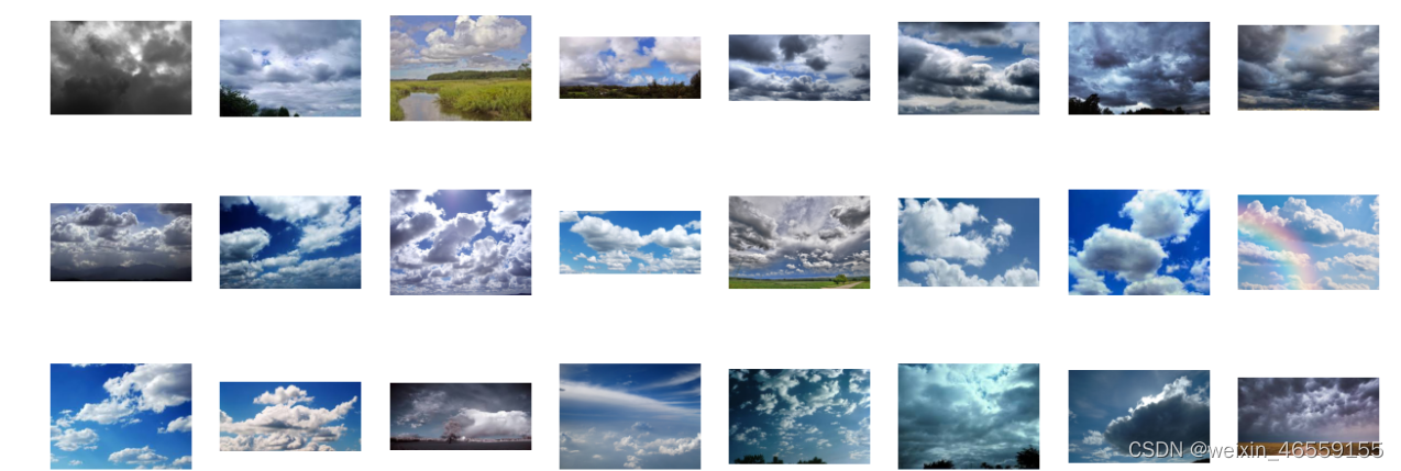
3.数据可视化

import matplotlib.pyplot as plt
from PIL import Image
def dispalyData(root):
    #获取文件夹中的所有图像文件
    imgs_files = [f for f in os.listdir(root) if f.endswith(('.png','.jpeg','.jpg'))]
    #创建matplotlib图像
    fig,axes = plt.subplots(3,8,figsize=(16,6))
    
    for ax,img_file in zip(axes.flat,imgs_files):
        img_path = os.path.join(root,img_file)
        img = Image.open(img_path)
        ax.imshow(img)
        ax.axis('off')
        
    plt.show()
        
root = r'F:\Netural_work_Data\P3_data\cloudy'
dispalyData(root)

4.加载数据

def LoadData(train_ds, test_ds,batch_size):
    train_dl = torch.utils.data.DataLoader(train_ds,
                                          batch_size=batch_size,
                                          shuffle=True,
                                          num_workers=2)
    test_dl  = torch.utils.data.DataLoader(test_ds,
                                          batch_size=batch_size,
                                          shuffle=True,
                                          num_workers=2)
    for X,y in train_dl:
        print('shape of X[N,C,H,W]:',X.shape)
        print('shape of y:',y.shape,y.dtype)
        break
    
    return(train_dl,test_dl)

batch_size = 2
train_dl,test_dl = LoadData(train_dataset,test_dataset,batch_size)

shape of X[N,C,H,W]: torch.Size([2, 3, 224, 224])
shape of y: torch.Size([2]) torch.int64

二、搭建包含C3模块的模型

YOLOV5模型相对于之前搭建的简单的CNN网络模型，VGG-16模型都更为复杂

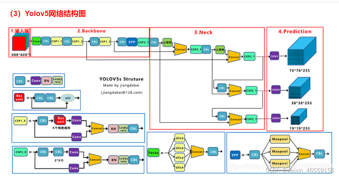以上为参考Yolov3、v4、v5、Yolox模型权重及网络结构图资源下载_yolov3模型下载-CSDN博客Yolov5网络结构图

我们对C3板块进行详解

1.antopad

import torch.nn.functional as F

def autopad(k, p=None, d=1):  # kernel, padding, dilation
    # Pad to 'same' shape outputs
    if d > 1:
        k = d * (k - 1) + 1 if isinstance(k, int) else [d * (x - 1) + 1 for x in k]  # actual kernel-size
    if p is None:
        p = k // 2 if isinstance(k, int) else [x // 2 for x in k]  # auto-pad
    return p

功能：为卷积或池化自动padding，可根据卷积核大小k自动计算卷积核padding数
用于Conv函数和Classify函数中
参数：k--卷积核大小
p--自动计算的需要pad值（）
d--膨胀标记

2.Conv

class Conv(nn.Module):
    default_act = nn.SiLU()# default activation 默认为SiLU激活函数
    
    # Standard convolution with args(ch_in, ch_out, kernel, stride, padding, groups, dilation, activation)
    def __init__(self,c1,c2,k=1,s=1,p=None,g=1,d=1,act=True):
        super().__init__()
        self.conv = nn.Conv2d(c1, c2, k, s, autopad(k, p, d), groups=g, dilation=d, bias=False)
        self.bn   = nn.BatchNorm2d(c2)
        self.act = self.default_act if act is True else act if isinstance(act, nn.Module) else nn.Identity()
        
    def forward(self,x):
        return self.act(self.bn(self.conv(x)))

该模块是网络中最基本的组件，为标准卷积层，由卷积层+BN层+激活函数组成，如下图所示。很多深度学习网络中的Conv层基本上是这样的组成，只是在激活函数上有所不同。

该模块在Focus、Bottleneck、BottleneckCSP、C3、SPP、DWConv、TransformerBloc等模块中调用
标准卷积 conv+BN+act

参数：c1 -- 输入channel值
c2 -- 输出channel值
k -- 卷积核size
s -- 卷积步长stride
p -- 卷积padding,通常为None,通过autopad自动计算需要pad的padding数
g -- 卷积的groups数，1为普通卷积，>1则为深度可分离卷积
act-- 激活函数类型，True就是默认激活函数SiLU()；
False就是不使用激活函数；
类型是nn.Module就使用传进来的激活函数类型；

3.Bottleneck

class Bottleneck(nn.Module):
    def __init__(self, c1, c2, shortcut=True, g=1, e=0.5):  # ch_in, ch_out, shortcut, groups, expansion
        super().__init__()
        c_ = int(c2 * e)  # hidden channels
        self.cv1 = Conv(c1, c_, 1, 1) # 1*1卷积
        self.cv2 = Conv(c_, c2, 3, 1, g=g) # 3*3卷积
        self.add = shortcut and c1 == c2 #shortcut为True，并且输入输出的channel大小一样才能进行add操作

    def forward(self,x):
        return x + self.cv2(self.cv1(x)) if self.add else self.cv2(self.cv1(x))

Bottleneck的模型结构如下图所示，当Shotcut=True（注意：具体代码里的条件为Shotcut and c1==c2）时，其网络结构类似残差网络，将输入input与两次Conv后的结构进行相加，否则不进行add操作。

在BottleneckCSP和yolo.py的parse_model函数中被调用
c1 -- 第一个卷积的输入channel
c2 -- 第二个卷积的输出channel
shortcut -- bool值，是否有shortcut连接，默认True
g -- 卷积分组的个数，=1普通卷积，>1深度可分离卷积
e -- 为bottleneck结构中的瓶颈部分的通道膨胀率（expansion ratio),使用0.5即为输入的1/2, e为控制瓶颈的参数，e越小则瓶颈越窄，瓶颈是指经过一个Conv将通道数缩小，然后再通过一个Conv变成原来的通道数，而e就是控制这个窄度的
e*c2就是第一个卷积的输出channel，也是第二个卷积的输入channel。

这里的瓶颈层，瓶颈主要体现在通道数channel上面！
一般1*1卷积具有很强的灵活性，这里用于降低通道数，如上面的膨胀率为0.5，
若输入通道为640，那么经过1*1的卷积层之后变为320；
经过3*3之后变为输出的通道数，这样参数量会大量减少
这里的shortcut即为图中的虚线，在实际中，shortcut（捷径）不一定是上面都不操作，
也有可能有卷积处理，但此时，另一只一般是多个ReNet模块串联而成。
而这里的shortcut也成为了identity分支，可以理解为恒等映射，
另一个分支被称为残差分支（Residual分支）
我们经常使用的残差分支实际上是1*1+3*3+1*1结构

4.C3

class C3(nn.Module):
    def __init__(self, c1, c2, n=1, shortcut=True, g=1, e=0.5):  # ch_in, ch_out, number, shortcut, groups, expansion
        super().__init__()
        c_ = int(c2 * e)  # hidden channels
        self.cv1 = Conv(c1, c_, 1, 1)
        self.cv2 = Conv(c1, c_, 1, 1)
        self.cv3 = Conv(2 * c_, c2, 1)  # optional act=FReLU(c2)
        self.m = nn.Sequential(*(Bottleneck(c_, c_, shortcut, g, e=1.0) for _ in range(n)))

    def forward(self,x):
        return self.cv3(torch.cat((self.m(self.cv1(x)),self.cv2(x)),dim=1))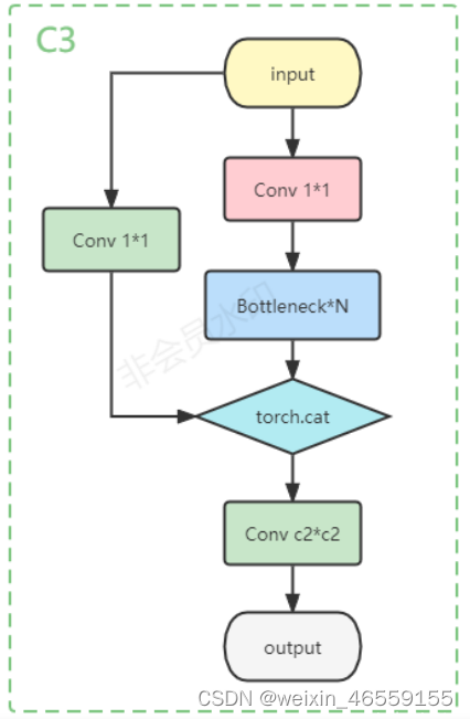

以上是C3的网络结构图，从结构中可以看出它和Bottleneck的结构非常相似，它是Bottleneck的优化版本，比Bottleneck更简单、快速和轻量，而其实现的功能却基本上相差无几。

在C3TR模块和yolo.py的parse_model模块调用
参数:c1 -- 整个BottleneckCSP的输入channel
c2 -- 整个BottleneckCSP的输出channel
n -- 有n个Bottleneck
shortcut -- bool Bottleneck中是否有shortcut，默认True
g -- Bottleneck中的3x3卷积类型 =1普通卷积 >1深度可分离卷积
e -- expansion ratio c2xe=中间其他所有层的卷积核个数/中间所有层的输入输出channel数

class model_K(nn.Module):
    def __init__(self):
        super(model_K, self).__init__()
        #卷积模块
        self.Conv = Conv(3, 32, 3, 2)
        #C3_1模块
        self.C3_1  = C3(32, 64, 3, 2) 
        
        # 全连接网络层，用于分类
        self.classifier = nn.Sequential(
            nn.Linear(in_features=802816, out_features=100),
            nn.ReLU(),
            nn.Linear(in_features=100, out_features=4)
        )
    
    def forward(self,x):
        x = self.Conv(x)
        x = self.C3_1(x)
        x = torch.flatten(x, start_dim=1)
        x = self.classifier(x)
        
        return x

device = "cuda" if torch.cuda.is_available() else "cpu"
print("Using {} device".format(device))
    
model = model_K().to(device)
model

model_K(
  (Conv): Conv(
    (conv): Conv2d(3, 32, kernel_size=(3, 3), stride=(2, 2), padding=(1, 1), bias=False)
    (bn): BatchNorm2d(32, eps=1e-05, momentum=0.1, affine=True, track_running_stats=True)
    (act): SiLU()
  )
  (C3_1): C3(
    (cv1): Conv(
      (conv): Conv2d(32, 32, kernel_size=(1, 1), stride=(1, 1), bias=False)
      (bn): BatchNorm2d(32, eps=1e-05, momentum=0.1, affine=True, track_running_stats=True)
      (act): SiLU()
    )
    (cv2): Conv(
      (conv): Conv2d(32, 32, kernel_size=(1, 1), stride=(1, 1), bias=False)
      (bn): BatchNorm2d(32, eps=1e-05, momentum=0.1, affine=True, track_running_stats=True)
      (act): SiLU()
    )
    (cv3): Conv(
      (conv): Conv2d(64, 64, kernel_size=(1, 1), stride=(1, 1), bias=False)
      (bn): BatchNorm2d(64, eps=1e-05, momentum=0.1, affine=True, track_running_stats=True)
      (act): SiLU()
    )
    (m): Sequential(
      (0): Bottleneck(
        (cv1): Conv(
          (conv): Conv2d(32, 32, kernel_size=(1, 1), stride=(1, 1), bias=False)
          (bn): BatchNorm2d(32, eps=1e-05, momentum=0.1, affine=True, track_running_stats=True)
          (act): SiLU()
        )
        (cv2): Conv(
          (conv): Conv2d(32, 32, kernel_size=(3, 3), stride=(1, 1), padding=(1, 1), bias=False)
          (bn): BatchNorm2d(32, eps=1e-05, momentum=0.1, affine=True, track_running_stats=True)
          (act): SiLU()
        )
      )
      (1): Bottleneck(
        (cv1): Conv(
          (conv): Conv2d(32, 32, kernel_size=(1, 1), stride=(1, 1), bias=False)
          (bn): BatchNorm2d(32, eps=1e-05, momentum=0.1, affine=True, track_running_stats=True)
          (act): SiLU()
        )
        (cv2): Conv(
          (conv): Conv2d(32, 32, kernel_size=(3, 3), stride=(1, 1), padding=(1, 1), bias=False)
          (bn): BatchNorm2d(32, eps=1e-05, momentum=0.1, affine=True, track_running_stats=True)
          (act): SiLU()
        )
      )
      (2): Bottleneck(
        (cv1): Conv(
          (conv): Conv2d(32, 32, kernel_size=(1, 1), stride=(1, 1), bias=False)
          (bn): BatchNorm2d(32, eps=1e-05, momentum=0.1, affine=True, track_running_stats=True)
          (act): SiLU()
        )
        (cv2): Conv(
          (conv): Conv2d(32, 32, kernel_size=(3, 3), stride=(1, 1), padding=(1, 1), bias=False)
          (bn): BatchNorm2d(32, eps=1e-05, momentum=0.1, affine=True, track_running_stats=True)
          (act): SiLU()
        )
      )
    )
  )
  (classifier): Sequential(
    (0): Linear(in_features=802816, out_features=100, bias=True)
    (1): ReLU()
    (2): Linear(in_features=100, out_features=4, bias=True)
  )
)

import torchsummary as summary
summary.summary(model, (3, 224, 224))

----------------------------------------------------------------
        Layer (type)               Output Shape         Param #
================================================================
            Conv2d-1         [-1, 32, 112, 112]             864
       BatchNorm2d-2         [-1, 32, 112, 112]              64
              SiLU-3         [-1, 32, 112, 112]               0
              SiLU-4         [-1, 32, 112, 112]               0
              SiLU-5         [-1, 32, 112, 112]               0
              SiLU-6         [-1, 32, 112, 112]               0
              SiLU-7         [-1, 32, 112, 112]               0
              SiLU-8         [-1, 32, 112, 112]               0
              SiLU-9         [-1, 32, 112, 112]               0
             SiLU-10         [-1, 32, 112, 112]               0
             SiLU-11         [-1, 32, 112, 112]               0
             SiLU-12         [-1, 32, 112, 112]               0
             Conv-13         [-1, 32, 112, 112]               0
           Conv2d-14         [-1, 32, 112, 112]           1,024
      BatchNorm2d-15         [-1, 32, 112, 112]              64
             SiLU-16         [-1, 32, 112, 112]               0
             SiLU-17         [-1, 32, 112, 112]               0
             SiLU-18         [-1, 32, 112, 112]               0
             SiLU-19         [-1, 32, 112, 112]               0
             SiLU-20         [-1, 32, 112, 112]               0
             SiLU-21         [-1, 32, 112, 112]               0
             SiLU-22         [-1, 32, 112, 112]               0
             SiLU-23         [-1, 32, 112, 112]               0
             SiLU-24         [-1, 32, 112, 112]               0
             SiLU-25         [-1, 32, 112, 112]               0
             Conv-26         [-1, 32, 112, 112]               0
           Conv2d-27         [-1, 32, 112, 112]           1,024
      BatchNorm2d-28         [-1, 32, 112, 112]              64
             SiLU-29         [-1, 32, 112, 112]               0
             SiLU-30         [-1, 32, 112, 112]               0
             SiLU-31         [-1, 32, 112, 112]               0
             SiLU-32         [-1, 32, 112, 112]               0
             SiLU-33         [-1, 32, 112, 112]               0
             SiLU-34         [-1, 32, 112, 112]               0
             SiLU-35         [-1, 32, 112, 112]               0
             SiLU-36         [-1, 32, 112, 112]               0
             SiLU-37         [-1, 32, 112, 112]               0
             SiLU-38         [-1, 32, 112, 112]               0
             Conv-39         [-1, 32, 112, 112]               0
           Conv2d-40         [-1, 32, 112, 112]           9,216
      BatchNorm2d-41         [-1, 32, 112, 112]              64
             SiLU-42         [-1, 32, 112, 112]               0
             SiLU-43         [-1, 32, 112, 112]               0
             SiLU-44         [-1, 32, 112, 112]               0
             SiLU-45         [-1, 32, 112, 112]               0
             SiLU-46         [-1, 32, 112, 112]               0
             SiLU-47         [-1, 32, 112, 112]               0
             SiLU-48         [-1, 32, 112, 112]               0
             SiLU-49         [-1, 32, 112, 112]               0
             SiLU-50         [-1, 32, 112, 112]               0
             SiLU-51         [-1, 32, 112, 112]               0
             Conv-52         [-1, 32, 112, 112]               0
       Bottleneck-53         [-1, 32, 112, 112]               0
           Conv2d-54         [-1, 32, 112, 112]           1,024
      BatchNorm2d-55         [-1, 32, 112, 112]              64
             SiLU-56         [-1, 32, 112, 112]               0
             SiLU-57         [-1, 32, 112, 112]               0
             SiLU-58         [-1, 32, 112, 112]               0
             SiLU-59         [-1, 32, 112, 112]               0
             SiLU-60         [-1, 32, 112, 112]               0
             SiLU-61         [-1, 32, 112, 112]               0
             SiLU-62         [-1, 32, 112, 112]               0
             SiLU-63         [-1, 32, 112, 112]               0
             SiLU-64         [-1, 32, 112, 112]               0
             SiLU-65         [-1, 32, 112, 112]               0
             Conv-66         [-1, 32, 112, 112]               0
           Conv2d-67         [-1, 32, 112, 112]           9,216
      BatchNorm2d-68         [-1, 32, 112, 112]              64
             SiLU-69         [-1, 32, 112, 112]               0
             SiLU-70         [-1, 32, 112, 112]               0
             SiLU-71         [-1, 32, 112, 112]               0
             SiLU-72         [-1, 32, 112, 112]               0
             SiLU-73         [-1, 32, 112, 112]               0
             SiLU-74         [-1, 32, 112, 112]               0
             SiLU-75         [-1, 32, 112, 112]               0
             SiLU-76         [-1, 32, 112, 112]               0
             SiLU-77         [-1, 32, 112, 112]               0
             SiLU-78         [-1, 32, 112, 112]               0
             Conv-79         [-1, 32, 112, 112]               0
       Bottleneck-80         [-1, 32, 112, 112]               0
           Conv2d-81         [-1, 32, 112, 112]           1,024
      BatchNorm2d-82         [-1, 32, 112, 112]              64
             SiLU-83         [-1, 32, 112, 112]               0
             SiLU-84         [-1, 32, 112, 112]               0
             SiLU-85         [-1, 32, 112, 112]               0
             SiLU-86         [-1, 32, 112, 112]               0
             SiLU-87         [-1, 32, 112, 112]               0
             SiLU-88         [-1, 32, 112, 112]               0
             SiLU-89         [-1, 32, 112, 112]               0
             SiLU-90         [-1, 32, 112, 112]               0
             SiLU-91         [-1, 32, 112, 112]               0
             SiLU-92         [-1, 32, 112, 112]               0
             Conv-93         [-1, 32, 112, 112]               0
           Conv2d-94         [-1, 32, 112, 112]           9,216
      BatchNorm2d-95         [-1, 32, 112, 112]              64
             SiLU-96         [-1, 32, 112, 112]               0
             SiLU-97         [-1, 32, 112, 112]               0
             SiLU-98         [-1, 32, 112, 112]               0
             SiLU-99         [-1, 32, 112, 112]               0
            SiLU-100         [-1, 32, 112, 112]               0
            SiLU-101         [-1, 32, 112, 112]               0
            SiLU-102         [-1, 32, 112, 112]               0
            SiLU-103         [-1, 32, 112, 112]               0
            SiLU-104         [-1, 32, 112, 112]               0
            SiLU-105         [-1, 32, 112, 112]               0
            Conv-106         [-1, 32, 112, 112]               0
      Bottleneck-107         [-1, 32, 112, 112]               0
          Conv2d-108         [-1, 32, 112, 112]           1,024
     BatchNorm2d-109         [-1, 32, 112, 112]              64
            SiLU-110         [-1, 32, 112, 112]               0
            SiLU-111         [-1, 32, 112, 112]               0
            SiLU-112         [-1, 32, 112, 112]               0
            SiLU-113         [-1, 32, 112, 112]               0
            SiLU-114         [-1, 32, 112, 112]               0
            SiLU-115         [-1, 32, 112, 112]               0
            SiLU-116         [-1, 32, 112, 112]               0
            SiLU-117         [-1, 32, 112, 112]               0
            SiLU-118         [-1, 32, 112, 112]               0
            SiLU-119         [-1, 32, 112, 112]               0
            Conv-120         [-1, 32, 112, 112]               0
          Conv2d-121         [-1, 64, 112, 112]           4,096
     BatchNorm2d-122         [-1, 64, 112, 112]             128
            SiLU-123         [-1, 64, 112, 112]               0
            SiLU-124         [-1, 64, 112, 112]               0
            SiLU-125         [-1, 64, 112, 112]               0
            SiLU-126         [-1, 64, 112, 112]               0
            SiLU-127         [-1, 64, 112, 112]               0
            SiLU-128         [-1, 64, 112, 112]               0
            SiLU-129         [-1, 64, 112, 112]               0
            SiLU-130         [-1, 64, 112, 112]               0
            SiLU-131         [-1, 64, 112, 112]               0
            SiLU-132         [-1, 64, 112, 112]               0
            Conv-133         [-1, 64, 112, 112]               0
              C3-134         [-1, 64, 112, 112]               0
          Linear-135                  [-1, 100]      80,281,700
            ReLU-136                  [-1, 100]               0
          Linear-137                    [-1, 4]             404
================================================================
Total params: 80,320,536
Trainable params: 80,320,536
Non-trainable params: 0
----------------------------------------------------------------
Input size (MB): 0.57
Forward/backward pass size (MB): 453.25
Params size (MB): 306.40
Estimated Total Size (MB): 760.22

三、训练模型

1.编写训练函数

def train(dataloader,model,optimizer,loss_fn):
    size = len(dataloader.dataset)
    num_batches = len(dataloader)
    
    train_loss,train_acc = 0,0
    
    for X,y in dataloader:
        X,y = X.to(device),y.to(device)
        
        #计算误差
        pred = model(X)
        loss = loss_fn(pred,y)
        
        #反向传播
        optimizer.zero_grad()
        loss.backward()
        optimizer.step()
        
        #记录loss与acc
        train_loss += loss.item()
        train_acc  += (pred.argmax(1) == y).type(torch.float).sum().item()
    
    train_loss /= num_batches
    train_acc  /= size
    
    return train_acc,train_loss

2.编写测试函数

def test(dataloader,model,loss_fn):
    size = len(dataloader.dataset)
    num_batches = len(dataloader)
    
    test_loss, test_acc = 0,0
    
    #当不训练时，梯度停止更新
    with torch.no_grad():
        for imgs,target in dataloader:
            imgs,target = imgs.to(device),target.to(device)
            
            #计算loss和acc
            target_pred = model(imgs)
            loss        = loss_fn(target_pred,target)
            
            test_loss  += loss.item()
            test_acc   += (target_pred.argmax(1) == target).type(torch.float).sum().item()
            
        test_acc  /= size
        test_loss /= num_batches
       
        
    return test_acc,test_loss

3.正式训练&设置超参数&保存最近模型

import time
import copy

'''设置超参数'''
start_epoch = 0
epochs = 50
learn_rate = 1e-4
loss_fn = nn.CrossEntropyLoss()
optimizer = torch.optim.Adam(model.parameters(),lr=learn_rate)
type(optimizer)
lambda1 = lambda epoch:0.92**(epoch//4)
scheduler = torch.optim.lr_scheduler.LambdaLR(optimizer,lr_lambda=lambda1)

train_loss = []
train_acc  = []
test_loss  = []
test_acc   = []
epoch_best_acc = 0

'''加载之前的模型'''
if not os.path.exists(output) or not os.path.isdir(output):
    os.makedirs(output)
if start_epoch > 0:
    resumeFile = os.path.join(output, 'epoch'+str(start_epoch)+'.pkl')
    if not os.path.exists(resumeFile) or not os.path.isfile(resumeFile):
        start_epoch = 0 
    else:
        model.load_state_dict(torch.load(resumeFile))

'''开始训练'''
print('\nStarting Training...')
best_model= None
for epoch in range(start_epoch, epochs):
    model.train()
    epoch_train_acc,epoch_train_loss = train(train_dl,model,optimizer,loss_fn)
    scheduler.step()
    
    model.eval()
    epoch_test_acc,epoch_test_loss = test(test_dl,model,loss_fn)
    
    train_acc.append(epoch_train_acc)
    train_loss.append(epoch_train_loss)
    test_acc.append(epoch_test_acc)
    test_loss.append(epoch_test_loss)

    lr = optimizer.state_dict()['param_groups'][0]['lr']
    
    template = ('Epoch:{:2d}, Train_acc:{:.1f}%, Train_loss:{:.3f}, Test_acc:{:.1f}%, Test_loss:{:.3f}, Lr:{:.2E}')
    print(time.strftime('[%Y-%m-%d %H:%M:%S]'), template.format(epoch+1, epoch_train_acc*100, epoch_train_loss, epoch_test_acc*100, epoch_test_loss, lr))

    # 保存最佳模型
    if epoch_test_acc>epoch_best_acc:
        ''' 保存最优模型参数 '''
        epoch_best_acc = epoch_test_acc
        best_model = copy.deepcopy(model)
        print(('acc = {:.1f}%, saving model to best.pkl').format(epoch_best_acc*100))
        saveFile = os.path.join(output, 'best.pkl')
        torch.save(best_model.state_dict(), saveFile)
print('Done\n')


''' 保存最新模型参数 '''
saveFile = os.path.join(output, 'epoch'+str(epochs)+'.pkl')
torch.save(model.state_dict(), saveFile)

Starting Training...
[2023-12-04 17:58:47] Epoch: 1, Train_acc:92.0%, Train_loss:0.459, Test_acc:80.0%, Test_loss:2.881, Lr:1.00E-04
acc = 80.0%, saving model to best.pkl
[2023-12-04 17:59:36] Epoch: 2, Train_acc:94.7%, Train_loss:0.226, Test_acc:87.6%, Test_loss:1.315, Lr:1.00E-04
acc = 87.6%, saving model to best.pkl
[2023-12-04 18:00:25] Epoch: 3, Train_acc:94.3%, Train_loss:0.340, Test_acc:89.3%, Test_loss:1.789, Lr:1.00E-04
acc = 89.3%, saving model to best.pkl
[2023-12-04 18:01:14] Epoch: 4, Train_acc:97.8%, Train_loss:0.170, Test_acc:86.7%, Test_loss:3.846, Lr:9.20E-05
[2023-12-04 18:02:01] Epoch: 5, Train_acc:97.7%, Train_loss:0.119, Test_acc:80.9%, Test_loss:3.275, Lr:9.20E-05
[2023-12-04 18:02:48] Epoch: 6, Train_acc:99.0%, Train_loss:0.033, Test_acc:88.0%, Test_loss:0.964, Lr:9.20E-05
[2023-12-04 18:03:35] Epoch: 7, Train_acc:98.0%, Train_loss:0.082, Test_acc:85.3%, Test_loss:1.708, Lr:9.20E-05
[2023-12-04 18:04:22] Epoch: 8, Train_acc:99.1%, Train_loss:0.031, Test_acc:88.9%, Test_loss:1.371, Lr:8.46E-05
[2023-12-04 18:05:10] Epoch: 9, Train_acc:99.6%, Train_loss:0.024, Test_acc:87.6%, Test_loss:1.418, Lr:8.46E-05
[2023-12-04 18:05:58] Epoch:10, Train_acc:98.3%, Train_loss:0.117, Test_acc:88.4%, Test_loss:1.264, Lr:8.46E-05
[2023-12-04 18:06:43] Epoch:11, Train_acc:99.0%, Train_loss:0.061, Test_acc:86.7%, Test_loss:2.695, Lr:8.46E-05
[2023-12-04 18:07:28] Epoch:12, Train_acc:98.6%, Train_loss:0.103, Test_acc:86.2%, Test_loss:1.930, Lr:7.79E-05
[2023-12-04 18:08:13] Epoch:13, Train_acc:98.1%, Train_loss:0.141, Test_acc:85.3%, Test_loss:1.868, Lr:7.79E-05
[2023-12-04 18:08:57] Epoch:14, Train_acc:99.1%, Train_loss:0.053, Test_acc:90.2%, Test_loss:1.508, Lr:7.79E-05
acc = 90.2%, saving model to best.pkl
[2023-12-04 18:09:43] Epoch:15, Train_acc:99.3%, Train_loss:0.022, Test_acc:90.7%, Test_loss:1.702, Lr:7.79E-05
acc = 90.7%, saving model to best.pkl
[2023-12-04 18:10:28] Epoch:16, Train_acc:99.6%, Train_loss:0.028, Test_acc:87.1%, Test_loss:2.031, Lr:7.16E-05
[2023-12-04 18:11:14] Epoch:17, Train_acc:99.7%, Train_loss:0.022, Test_acc:89.3%, Test_loss:1.690, Lr:7.16E-05
[2023-12-04 18:12:00] Epoch:18, Train_acc:99.6%, Train_loss:0.012, Test_acc:91.6%, Test_loss:1.847, Lr:7.16E-05
acc = 91.6%, saving model to best.pkl
...
[2023-12-04 18:29:43] Epoch:42, Train_acc:100.0%, Train_loss:0.000, Test_acc:90.2%, Test_loss:2.933, Lr:4.34E-05
[2023-12-04 18:30:27] Epoch:43, Train_acc:100.0%, Train_loss:0.000, Test_acc:90.7%, Test_loss:2.669, Lr:4.34E-05
[2023-12-04 18:31:11] Epoch:44, Train_acc:99.9%, Train_loss:0.001, Test_acc:89.3%, Test_loss:3.004, Lr:4.00E-05
[2023-12-04 18:31:55] Epoch:45, Train_acc:99.8%, Train_loss:0.005, Test_acc:86.7%, Test_loss:2.610, Lr:4.00E-05
[2023-12-04 18:32:39] Epoch:46, Train_acc:100.0%, Train_loss:0.001, Test_acc:87.6%, Test_loss:2.658, Lr:4.00E-05
[2023-12-04 18:33:24] Epoch:47, Train_acc:100.0%, Train_loss:0.000, Test_acc:89.8%, Test_loss:2.059, Lr:4.00E-05
[2023-12-04 18:34:08] Epoch:48, Train_acc:100.0%, Train_loss:0.000, Test_acc:89.3%, Test_loss:2.360, Lr:3.68E-05
[2023-12-04 18:34:52] Epoch:49, Train_acc:100.0%, Train_loss:0.000, Test_acc:87.1%, Test_loss:2.904, Lr:3.68E-05
[2023-12-04 18:35:36] Epoch:50, Train_acc:100.0%, Train_loss:0.000, Test_acc:88.9%, Test_loss:3.139, Lr:3.68E-05
Dones

四、结果可视化

''' 结果可视化 '''
def displayResult(train_acc, test_acc, train_loss, test_loss, start_epoch, epochs, output=''):
 
    plt.rcParams['font.sans-serif']    = ['SimHei']  # 用来正常显示中文标签
    plt.rcParams['axes.unicode_minus'] = False       # 用来正常显示负号
    plt.rcParams['figure.dpi']         = 100         # 分辨率
    
    epochs_range = range(start_epoch, epochs)
    
    plt.figure('Result Visualization', figsize=(12, 3))
    plt.subplot(1, 2, 1)
    
    plt.plot(epochs_range, train_acc, label='Training Accuracy')
    plt.plot(epochs_range, test_acc, label='Test Accuracy')
    plt.legend(loc='lower right')
    plt.title('Training and Validation Accuracy')
    
    plt.subplot(1, 2, 2)
    plt.plot(epochs_range, train_loss, label='Training Loss')
    plt.plot(epochs_range, test_loss, label='Test Loss')
    plt.legend(loc='upper right')
    plt.title('Training and Validation Loss')
    plt.savefig(os.path.join(output, 'AccuracyLoss.png'))
    plt.show()
 
''' 绘制准确率&损失率曲线图 '''
displayResult(train_acc, test_acc, train_loss, test_loss, start_epoch, epochs, output)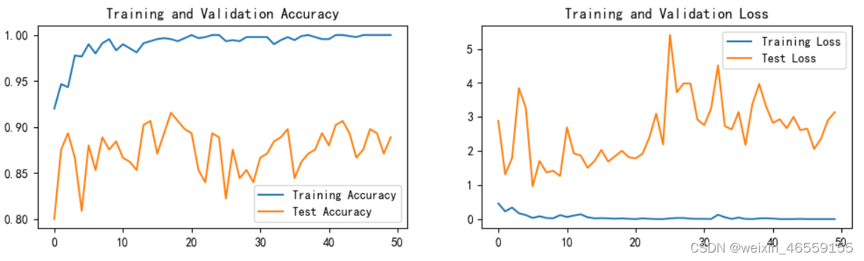

五、加载指定图片并进行预测

''' 预测函数 '''
import PIL
from PIL import Image
 
def predict(model, img_path):
    img = Image.open(img_path)
    test_transforms = torchvision.transforms.Compose([
        torchvision.transforms.Resize([224, 224]),  # 将输入图片resize成统一尺寸
        torchvision.transforms.ToTensor(),          # 将PIL Image或numpy.ndarray转换为tensor，并归一化到[0,1]之间
        torchvision.transforms.Normalize(           # 标准化处理-->转换为标准正太分布（高斯分布），使模型更容易收敛
            mean=[0.485, 0.456, 0.406], 
            std=[0.229, 0.224, 0.225])  # 其中 mean=[0.485,0.456,0.406]与std=[0.229,0.224,0.225] 从数据集中随机抽样计算得到的。
    ])
    img = test_transforms(img)
    img = img.to(device).unsqueeze(0)
    output = model(img)
    #print(output.argmax(1))
    
    _, indices = torch.max(output, 1)
    percentage = torch.nn.functional.softmax(output, dim=1)[0] * 100
    perc = percentage[int(indices)].item()
    result = classeNames[indices]
    print('predicted:', result, perc)
 
 
if __name__=='__main__':
    classeNames = list({'Cloudy': 0, 'Rain': 1, 'Shine': 2, 'Sunrise': 3})
    num_classes = len(classeNames)
    
    device = torch.device("cuda" if torch.cuda.is_available() else "cpu")
    print("Using {} device\n".format(device))
    
    model = model_K().to(device)  # 加载自定义的model_K模型
    model.load_state_dict(torch.load(r'F:\model_param\p_8_model\best.pkl'))
    model.eval()
    
    img_path = r'F:\Netural_work_Data\P3_data\cloudy\cloudy1.jpg'
    predict(model, img_path)

Using cuda device
predicted: Cloudy 99.9995727539062

六、个人总结

1.这个YOLOv5模型结构比之前学的模型都要难，目前看了几篇博客，也只能算是刚刚了解，还得继续看

2.对比第三周构建简单的CNN来做天气预测，用YOLOv5做训练，accuracy上去了一些，但是并没有说达到95%以上这种精度，并且计算还很大，batch_size由设定的32改成了4才跑起来的，所以就这个问题而言，用YOLOv5，计算千万计的参数，但是得到的效果没有显著提升，所以模型的适用性到底怎么界定？

weixin_46559155

关注

38
点赞
踩
45

收藏

觉得还不错? 一键收藏
0
评论
365天深度学习训练营-第P8周：YOLOv5-C3模块实现

1.这个YOLOv5模型结构比之前学的模型都要难，目前看了几篇博客，也只能算是刚刚了解，还得继续看2.对比第三周构建简单的CNN来做天气预测，用YOLOv5做训练，accuracy上去了一些，但是并没有说达到95%以上这种精度，并且计算还很大，batch_size由设定的32改成了4才跑起来的，所以就这个问题而言，用YOLOv5，计算千万计的参数，但是得到的效果没有显著提升，所以模型的适用性到底怎么界定？
复制链接

扫一扫