数据分析项目-合集-day01

最新推荐文章于 2024-05-14 14:35:46 发布

weixin_47049321

最新推荐文章于 2024-05-14 14:35:46 发布

阅读量166

点赞数

文章标签：数据分析 python 数据挖掘

本文链接：https://blog.csdn.net/weixin_47049321/article/details/124637720

版权

提示：文章写完后，目录可以自动生成，如何生成可参考右边的帮助文档

数据分析项目-合集-day01

需求：股票分析
需求：双均线策略制定

需求：股票分析

使用tushare包获取某支股票历史行情数据。
输出该股票所有收盘比开盘上涨3%的日期。
输出该股票所有开盘比上日收盘跌幅超过2%的日期
假如我从2010年开始，每月第一个交易日买入1手股票，每年最后一个交易日卖出所有股票，到今天为止，我的收益如何？
tushare财经数据接口包
pip install tushare

import tushare as ts
import pandas as pd
from pandas import DataFrame,Series
import numpy as np

获取某只股票的历史行情数据

#code 字符串形式的股票代码
df=ts.get_k_data(code="600519",start="2000-01-01")
df

运行结果：


date	open	close	high	low	volume	code
0	2001-08-27	-91.359	-91.174	-90.778	-91.654	406318.00	600519
1	2001-08-28	-91.274	-90.941	-90.916	-91.341	129647.79	600519
2	2001-08-29	-90.920	-91.027	-90.916	-91.076	53252.75	600519
3	2001-08-30	-91.044	-90.899	-90.826	-91.094	48013.06	600519
4	2001-08-31	-90.890	-90.915	-90.806	-90.952	23231.48	600519
...	...	...	...	...	...	...	...
4939	2022-04-27	1767.120	1794.920	1810.000	1767.120	57402.00	600519
4940	2022-04-28	1793.000	1835.000	1845.000	1786.500	44010.00	600519
4941	2022-04-29	1836.000	1828.380	1849.000	1810.980	34885.00	600519
4942	2022-05-05	1830.000	1837.000	1870.000	1828.980	33661.00	600519
4943	2022-05-06	1814.990	1793.000	1819.000	1781.000	28596.00	600519
4944 rows × 7 columns

将互联网上获取的股票数据存储到本地

#调用to_xxx方法将df中的数据写入到本地进行存储
df.to_csv("./maotai.csv")

#将本地存储的数据读入到df

df=pd.read_csv("./maotai.csv")
df.head()

运行结果：


Unnamed: 0	date	open	close	high	low	volume	code
0	0	2001-08-27	-91.359	-91.174	-90.778	-91.654	406318.00	600519
1	1	2001-08-28	-91.274	-90.941	-90.916	-91.341	129647.79	600519
2	2	2001-08-29	-90.920	-91.027	-90.916	-91.076	53252.75	600519
3	3	2001-08-30	-91.044	-90.899	-90.826	-91.094	48013.06	600519
4	4	2001-08-31	-90.890	-90.915	-90.806	-90.952	23231.48	600519

需要对读取出来的数据进行相关的处理

删除df中指定的一列

axis输入0代表列，1代表行。但是对drop方法而言，正好是相反的

df.drop(labels="Unnamed: 0",axis=1,inplace=True)
df.head()

运行结果：

	date	open	close	high	low	volume	code
0	2001-08-27	-91.359	-91.174	-90.778	-91.654	406318.00	600519
1	2001-08-28	-91.274	-90.941	-90.916	-91.341	129647.79	600519
2	2001-08-29	-90.920	-91.027	-90.916	-91.076	53252.75	600519
3	2001-08-30	-91.044	-90.899	-90.826	-91.094	48013.06	600519
4	2001-08-31	-90.890	-90.915	-90.806	-90.952	23231.48	600519

查看每一列数据类型


df.info()

<class 'pandas.core.frame.DataFrame'>
RangeIndex: 4944 entries, 0 to 4943
Data columns (total 7 columns):
 #   Column  Non-Null Count  Dtype  
---  ------  --------------  -----  
 0   date    4944 non-null   object 
 1   open    4944 non-null   float64
 2   close   4944 non-null   float64
 3   high    4944 non-null   float64
 4   low     4944 non-null   float64
 5   volume  4944 non-null   float64
 6   code    4944 non-null   int64  
dtypes: float64(5), int64(1), object(1)
memory usage: 270.5+ KB

将date列转为时间序列类型

#由于后续很多操作需要用到日期

df["date"]=pd.to_datetime(df["date"])

#将date列作为源数据的行索引
df.set_index("date",inplace=True)

df.head()

运行结果：


open	close	high	low	volume	code
date						
2001-08-27	-91.359	-91.174	-90.778	-91.654	406318.00	600519
2001-08-28	-91.274	-90.941	-90.916	-91.341	129647.79	600519
2001-08-29	-90.920	-91.027	-90.916	-91.076	53252.75	600519
2001-08-30	-91.044	-90.899	-90.826	-91.094	48013.06	600519
2001-08-31	-90.890	-90.915	-90.806	-90.952	23231.48	600519

输出该股票所有收盘比开盘上涨3%的日期。

#伪代码： （收盘-开盘）/开盘 >0.03
(df["close"]-df["open"])/df["open"]>0.03

#在分析过程中产生的布尔值，则下一步马上将布尔运算作为源数据的行索引
    #如果布尔值作为df的行索引，则可以取出true对应的行数据，忽略false对应的行数据
df.loc[(df["close"]-df["open"])/df["open"]>0.03]#获取了True对应的行数据

df.loc[(df["close"]-df["open"])/df["open"]>0.03].index #df的行数据

运行结果：

DatetimeIndex(['2006-05-25', '2006-06-02', '2006-12-19', '2006-12-21',
               '2006-12-22', '2007-01-04', '2007-01-08', '2007-01-16',
               '2007-01-23', '2007-01-31',
               ...
               '2021-09-01', '2021-09-17', '2021-09-24', '2021-09-27',
               '2021-10-13', '2021-12-08', '2021-12-23', '2022-02-09',
               '2022-03-01', '2022-04-12'],
              dtype='datetime64[ns]', name='date', length=748, freq=None)

输出该股票所有开盘比上日收盘跌幅超过2%的日期

#伪代码： （开盘-前日收盘）/前日收盘 < -0.02
(df["open"]-df["close"].shift(1))/df["close"].shift(1)<-0.02
#将布尔值作为源数据的行索引取出True对应的行数据
df.loc[(df["open"]-df["close"].shift(1))/df["close"].shift(1)<-0.02]
#根据index取出满足条件的日期
df.loc[(df["open"]-df["close"].shift(1))/df["close"].shift(1)<-0.02].index

运行结果：

DatetimeIndex(['2006-02-13', '2006-04-17', '2006-04-18', '2006-04-19',
               '2006-04-20', '2006-05-25', '2006-05-30', '2006-12-27',
               '2007-01-04', '2007-01-22',
               ...
               '2020-03-23', '2020-10-26', '2021-02-26', '2021-03-04',
               '2021-04-28', '2021-08-20', '2021-11-01', '2022-03-14',
               '2022-03-15', '2022-03-28'],
              dtype='datetime64[ns]', name='date', length=378, freq=None)

需求：假如我从2010年开始，每月第一个交易日买入1手股票，每年最后一个交易日卖出所有股票，到今天为止，我的收益如何？
分析：
时间节点：2010-2022
一手股票：100支股票
买：
一个完整的年需要买入1200支股票

卖：
一个完整的年需要卖出1200支股票

买卖股票的单价：
开盘价

new_df=df["2010-01":"2022-04"]
new_df
运行结果：

open	close	high	low	volume	code
date						
2010-01-04	35.594	34.047	35.594	33.573	44304.88	600519
2010-01-05	34.835	33.671	35.219	33.340	31513.18	600519
2010-01-06	33.333	31.657	33.716	31.319	39889.03	600519
2010-01-07	31.657	29.373	31.980	27.991	48825.55	600519
2010-01-08	29.584	28.081	29.584	26.654	36702.09	600519
...	...	...	...	...	...	...
2022-04-25	1750.000	1708.000	1776.500	1702.000	53658.00	600519
2022-04-26	1703.330	1732.480	1748.980	1700.000	44564.00	600519
2022-04-27	1767.120	1794.920	1810.000	1767.120	57402.00	600519
2022-04-28	1793.000	1835.000	1845.000	1786.500	44010.00	600519
2022-04-29	1836.000	1828.380	1849.000	1810.980	34885.00	600519
2988 rows × 6 columns

买股票:找到每个月的第一个交易日对应的行数据（捕获到开盘价）==>>每月的第一行数据

#根据月份从原始数据中提取指定的数据
#每月第一个交易日对应的行数据
df_monthly=new_df.resample("M").first()#数据的重写取样
df_monthly
运行结果：

open	close	high	low	volume	code
date						
2010-01-31	35.594	34.047	35.594	33.573	44304.88	600519
2010-02-28	33.250	33.258	33.776	31.845	29655.94	600519
2010-03-31	31.424	31.267	32.176	31.079	21734.74	600519
2010-04-30	25.662	26.624	26.954	25.647	23980.83	600519
2010-05-31	2.529	3.017	3.708	1.702	23975.16	600519
...	...	...	...	...	...	...
2021-12-31	1950.000	1932.990	1959.950	1919.020	26254.00	600519
2022-01-31	2055.000	2051.230	2068.950	2014.000	33843.00	600519
2022-02-28	1900.990	1867.960	1913.560	1850.000	35150.00	600519
2022-03-31	1802.000	1858.480	1863.570	1802.000	47379.00	600519
2022-04-30	1729.940	1780.010	1793.000	1721.690	44862.00	600519
148 rows × 6 columns

#买入股票花费的总金额

cost=df_monthly["open"].sum()*100
cost
运行结果：
7779065.1

卖出股票到手的钱

#特殊情况：2022年买入的股票卖不出去
new_df.resample("A").last()
#将2022年最后一行切出去
df_yearly=new_df.resample("A").last()[:-1]
df_yearly
运行结果：
	open	close	high	low	volume	code
date						
2010-12-31	43.847	45.440	45.711	43.284	46084.0	600519
2011-12-31	68.243	68.739	70.044	66.011	29460.0	600519
2012-12-31	88.579	85.034	89.810	82.827	51914.0	600519
2013-12-31	20.074	23.694	24.463	18.834	57546.0	600519
2014-12-31	89.937	93.591	93.937	89.391	46269.0	600519
2015-12-31	143.406	143.376	144.686	143.006	19673.0	600519
2016-12-31	257.967	265.507	266.647	257.967	34687.0	600519
2017-12-31	656.144	635.634	664.644	629.744	76038.0	600519
2018-12-31	512.443	539.153	545.543	509.143	63678.0	600519
2019-12-31	1146.682	1146.682	1151.682	1140.192	22588.0	600519
2020-12-31	1921.707	1978.707	1979.687	1919.707	38860.0	600519
2021-12-31	2070.000	2050.000	2072.980	2028.000	29665.0	600519

卖出股票到手的钱

resv=df_yearly["open"].sum()*1200
resv
运行结果：
8422834.8

#最后手中剩余的股票需要估算其价值计算到总收益中
#使用昨天的收盘价作为剩余股票的单价
last_money=400*new_df["close"][-1]
last_money
运行结果：
731352.0

#计算总收益
resv+last_money-cost
运行结果：
1375121.7000000011

需求：双均线策略制定

使用tushare包获取某股票的历史行情数据

df=pd.read_csv('./maotai.csv').drop(labels="Unnamed: 0",axis=1)
df

运行结果：

date	open	close	high	low	volume	code
0	2001-08-27	-91.359	-91.174	-90.778	-91.654	406318.00	600519
1	2001-08-28	-91.274	-90.941	-90.916	-91.341	129647.79	600519
2	2001-08-29	-90.920	-91.027	-90.916	-91.076	53252.75	600519
3	2001-08-30	-91.044	-90.899	-90.826	-91.094	48013.06	600519
4	2001-08-31	-90.890	-90.915	-90.806	-90.952	23231.48	600519
...	...	...	...	...	...	...	...
4939	2022-04-27	1767.120	1794.920	1810.000	1767.120	57402.00	600519
4940	2022-04-28	1793.000	1835.000	1845.000	1786.500	44010.00	600519
4941	2022-04-29	1836.000	1828.380	1849.000	1810.980	34885.00	600519
4942	2022-05-05	1830.000	1837.000	1870.000	1828.980	33661.00	600519
4943	2022-05-06	1814.990	1793.000	1819.000	1781.000	28596.00	600519
4944 rows × 7 columns

#将date列转为时间序列且将其作为源数据的行索引
df["date"]=pd.to_datetime(df["date"])

df.set_index("date",inplace=True)
df.head()
运行结果：

open	close	high	low	volume	code
date						
2001-08-27	-91.359	-91.174	-90.778	-91.654	406318.00	600519
2001-08-28	-91.274	-90.941	-90.916	-91.341	129647.79	600519
2001-08-29	-90.920	-91.027	-90.916	-91.076	53252.75	600519
2001-08-30	-91.044	-90.899	-90.826	-91.094	48013.06	600519
2001-08-31	-90.890	-90.915	-90.806	-90.952	23231.48	600519

计算该股票的历史数据的5日均线和30日均线
什么是均线
对于每一个交易日，都可以计算出前N天的移动平均值，然后把这些移动平均值连起来，成为一条线，
就叫做N日移动平均线。移动平均线常用线有5天，10天，30天，60天，120天和240天的指标。
- 5天和10天的是短线操作的参照指标，叫日均线指标
- 30天和60天的是中期指标，叫季均线指标
- 120天和240天的是长期均线指标，叫年均线指标
均线计算方法：MA=（C1+C2+C3+…+Cn）/N , C:某日收盘价， N：移动平均周期（天数）

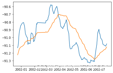
ma5=df["close"].rolling(5).mean()
ma30=df["close"].rolling(30).mean()

import matplotlib.pyplot as plt
%matplotlib inline
plt.plot(ma5[50:180])
plt.plot(ma30[50:180])

在这里插入图片描述

分析输出所有的金叉日期和死叉日期
股票分析技术中的金叉和死叉，可以解释为：
分析指标中的两根线，一根为短时间内的指标线，另一根为较长时间的指标线
如果短时间的指标线方向拐头向上，并且穿过了较长时间的指标线，这种状态叫“金叉”
如果短时间的指标线方向拐头向下，并且穿过了较长时间的指标线，这种状态叫“死叉”
一般情况下，出现金叉后，操作趋向买入；死叉则趋向卖出。当然，金叉和死叉是分析的指标之一，
要和其他很多指标配合使用，才能增加操作的正确性

# 删除ma5和ma30列中的NaN值，前30个.
# 同时df为了和ma5和ma30时间索引相同，也从后30个开始数
ma5=ma5[30:]
ma30=ma30[30:]
df=df[30:]

s1=ma5<ma30
s2=ma5>ma30

#s1从True变为False为金叉，s1从False变为True为死叉
death_ex=s1&s2.shift(1) #判定死叉的条件,(s1 与 “s2.向下移动1行”)
df.loc[death_ex] #死叉对应的行数据
death_date= df.loc[death_ex].index

death_date
运行结果：
DatetimeIndex(['2002-01-17', '2002-01-30', '2002-03-29', '2002-07-29',
               '2002-12-27', '2003-03-17', '2003-04-22', '2003-06-20',
               '2003-06-30', '2003-08-04',
               ...
               '2020-03-18', '2020-08-10', '2020-09-21', '2020-10-27',
               '2021-03-01', '2021-04-15', '2021-05-06', '2021-06-22',
               '2021-11-04', '2022-01-06'],
              dtype='datetime64[ns]', name='date', length=104, freq=None)


golden_ex=~s1|s2.shift(1) #判定金叉的条件(s1 或 “s2.向下移动1行”)
golden_date=df.loc[golden_ex].index

golden_date
运行结果：
DatetimeIndex(['2001-11-22', '2001-11-23', '2001-11-26', '2001-11-27',
               '2001-11-28', '2001-11-29', '2001-11-30', '2001-12-03',
               '2001-12-04', '2001-12-05',
               ...
               '2022-04-20', '2022-04-21', '2022-04-22', '2022-04-25',
               '2022-04-26', '2022-04-27', '2022-04-28', '2022-04-29',
               '2022-05-05', '2022-05-06'],
              dtype='datetime64[ns]', name='date', length=2983, freq=None)

在这里插入图片描述

weixin_47049321

关注

0
点赞
踩
0

收藏

觉得还不错? 一键收藏
打赏
0
评论
数据分析项目-合集-day01

提示：文章写完后，目录可以自动生成，如何生成可参考右边的帮助文档数据分析项目-合集-day01需求：股票分析需要对读取出来的数据进行相关的处理需求：双均线策略制定删除ma5和ma30列中的NaN值，前30个.同时df为了和ma5和ma30时间索引相同，也从后30个开始数需求：股票分析使用tushare包获取某支股票历史行情数据。输出该股票所有收盘比开盘上涨3%的日期。输出该股票所有开盘比上日收盘跌幅超过2%的日期假如我从2010年开始，每月第一个交易日买入1手股票，每年最后.
复制链接

扫一扫