diffusion models 扩散模型公式推导，原理分析与代码（一）

前言

近几年来，以对抗生成网络（GAN）和变分自编码器（VAE）为主流的生成模型一直作为研究的热点，这两种模型有各自的特点，也有其本身的原理特性所带来的不足，对这两种模型有过一定了解的一般会有这样的认知：以图像生成为例，GAN的优势在于可以生成更加逼真的图像，但是容易出现生成图大部分局限在同一个模式下，不能够很好的概括数据的分布，除此之外，GAN有时难以训练，一个好的GAN模型通常需要繁琐的参数调整，正则化等等。相对地，VAE这种以数据分布的对数似然（log-likelihood）为逼近目标的模式，要比GAN能够生成更加多样的图像，但在图像质量上还是逊色于GAN模型。
有没有模型可以两者兼得呢？
diffusion models似乎给这个目标带来了可能，这个模型的最初版本在2015年被提出，直到2020年的一篇论文对该模型做了大幅度的改进，扩散模型逐渐获得关注，这两年关于该模型的研究越来越多，尤其是openAI（就是那个开发chatGBT的公司）对扩散模型的改进做了一些标志性贡献，使这个模型有了一些品牌效应。
本文介绍扩散模型最初的两篇论文，包括公式推导，以及一些公式背后的物理直觉，最后尽可能的简单而全面的给出模型实现过程的程序。
论文：
《Deep Unsupervised Learning using Nonequilibrium Thermodynamics》
《Denoising Diffusion Probabilistic Models》

基本思想

对于一个数据集（数据分布为$p(\mathbf{x})$），如果以马尔科夫过程的形式不断添加高斯噪声，缓慢地破坏数据分布的结构，如果该过程足够缓慢，最后数据集的分布可以认为是一个均质的高斯分布（在各个维度都一样），这个过程也称为扩散。随后，给定一张完全从高斯分布中采样的图像，能否根据扩散过程的已知参数，反向推导出一开始的数据分布$p(\mathbf{x})$？
为了便于表示，我们将从原始数据分布扩散到完全的高斯噪声的过程称为前向扩散过程（forward diffusion process），将由高斯噪声反推到原始图像分布的过程称为反向扩散过程（reverse diffusion process）。

符号定义

将原始图像定义为${\mathbf{x}}_0$，扩散过程的$t$时刻对应的图像定义为${\mathbf{x}}_t$，从初始图像到完全扩散为高斯噪声所经历的时间为$T$，对应${\mathbf{x}}_T$，不同的论文中对$T$的设置有所不同，下图给出了一个形象化表示的示例：

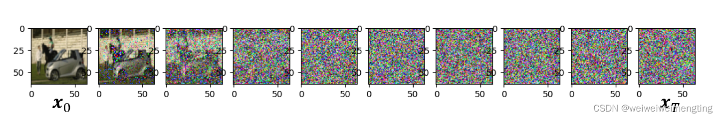
定义$q\left({\mathbf{x}}_t\mid {\mathbf{x}}_{t-1}\right)$为前向过程的转移概率分布，也就是说${\mathbf{x}}_{t-1}$总是对应噪声较少的图像，同时定义$p_{\theta }\left({\mathbf{x}}_{t-1}\mid {\mathbf{x}}_t\right)$为反向过程的转移概率分布，接下来，前向过程的转移分布的具体形式为：

$$q\left({\mathbf{x}}_t\mid {\mathbf{x}}_{t-1}\right)=\mathcal{N}\left({\mathbf{x}}_t;\sqrt{1-{\beta }_t}{\mathbf{x}}_{t-1},{\beta }_{t}I\right)$$

这个公式这样去理解，首先，${\mathbf{x}}_t$的分布可以写成是以${\mathbf{x}}_{t-1}$为条件的分布，这个分布是一个高斯的形式，它的均值为$\sqrt{1-{\beta }_t}{\mathbf{x}}_{t-1}$，方差为${\beta }_{t}I$，在马尔可夫过程中我们知道，给定一个状态的概率分布，通过转移概率分布可以计算出下一个状态的概率分布，这里的不同时刻的$x$就是不同的状态。
根据这个公式，如果要得到最终的$x_T$，我们需要将上面的公式不停迭代$T$次，实际上，有一种更直接的方法可以直接获得任意时刻$t$所对应的图像：
我们重新给出一个定义：
$$\begin{array}{rl}{\alpha }_t& =1-{\beta }_t\\ {\bar{\alpha }}_t& =\prod _{s=1}^t{a}_s\end{array}$$
接下来，用这个新的定义重写上式，已知$x_t$对应的高斯分布的均值和方差，通过重参数（reparameterization trick），可以将${\mathbf{x}}_t$表示成如下的形式：
$$\begin{array}{rl}{\mathbf{x}}_t& =\sqrt{1-{\beta }_t}{\mathbf{x}}_{t-1}+\sqrt{{\beta }_t}\mathbf{ϵ}\\ & =\sqrt{{\alpha }_t}{\mathbf{x}}_{t-1}+\sqrt{1-{\alpha }_t}\mathbf{ϵ}\end{array}$$
如果对重参数不懂的话可以查阅资料，这个很好理解，不做过多解释。$ϵ\sim \mathcal{N}(0,I),\mathcal{N}(\mu ,{\sigma }^2)=\mu +\sigma ϵ$。
另一方面，根据递推可以知道${\mathbf{x}}_{t-1}$和${\mathbf{x}}_{t-2}$的关系：
$${\mathbf{x}}_{t-1}=\sqrt{{\alpha }_{t-1}}{\mathbf{x}}_{t-2}+\sqrt{1-{\alpha }_{t-1}}\mathbf{ϵ}$$
为了避免混淆，我们暂时用${\mathbf{ϵ}}^{\ast }$表示$\mathcal{N}(0,I)$，代入上式，可以得到：
$$\begin{array}{rl}{\mathbf{x}}_t& =\sqrt{{\alpha }_t}{\mathbf{x}}_{t-1}+\sqrt{1-{\alpha }_t}{\mathbf{ϵ}}^{\ast }\\ & =\sqrt{{\alpha }_t}(\sqrt{{\alpha }_{t-1}}{\mathbf{x}}_{t-2}+\sqrt{1-{\alpha }_{t-1}}{\mathbf{ϵ}}^{\ast })+\sqrt{1-{\alpha }_t}{\mathbf{ϵ}}^{\ast }\\ & =\sqrt{{\alpha }_t}\sqrt{{\alpha }_{t-1}}{\mathbf{x}}_{t-2}+\sqrt{{\alpha }_t}\sqrt{1-{\alpha }_{t-1}}{\mathbf{ϵ}}^{\ast }+\sqrt{1-{\alpha }_t}{\mathbf{ϵ}}^{\ast }\end{array}$$
我们将后两项合并，带有权重的两个标准正太分布的和：
$$\begin{array}{rl}& \sqrt{{\alpha }_t}\sqrt{1-{\alpha }_{t-1}}{\mathbf{ϵ}}^{\ast }+\sqrt{1-{\alpha }_t}{\mathbf{ϵ}}^{\ast }\end{array}$$
已知$A=C\mathrm{I}+D\mathrm{I}$，那么${\sigma }_A^2={\sigma }_C^2+{\sigma }_D^2,{\mu }_A={\mu }_C+{\mu }_D$，所以上式对应的新的
$$\begin{array}{rl}{\sigma }^2& =(\sqrt{{\alpha }_t}\sqrt{1-{\alpha }_{t-1}}{)}^2+(\sqrt{1-{\alpha }_t}{)}^2\\ & ={\alpha }_t(1-{\alpha }_{t-1})+1-{\alpha }_t\\ & =1-{\alpha }_t{\alpha }_{t-1}\end{array}$$
写成一个新的高斯分布：
$$\begin{array}{rl}& \sqrt{{\alpha }_t}\sqrt{1-{\alpha }_{t-1}}{\mathbf{ϵ}}^{\ast }+\sqrt{1-{\alpha }_t}{\mathbf{ϵ}}^{\ast }\\ & =\sqrt{1-{\alpha }_t{\alpha }_{t-1}}{\mathbf{ϵ}}^{\ast }\end{array}$$
我们将${\mathbf{ϵ}}^{\ast }$换回$\mathbf{ϵ}$，带入${\mathbf{x}}_t$，可以得到：
$$\begin{array}{rl}{\mathbf{x}}_t& =\sqrt{{\alpha }_t}{\mathbf{x}}_{t-1}+\sqrt{1-{\alpha }_t}{\mathbf{ϵ}}^{\ast }\\ & =\sqrt{{\alpha }_t}\sqrt{{\alpha }_{t-1}}{\mathbf{x}}_{t-2}+\sqrt{1-{\alpha }_t{\alpha }_{t-1}}\mathbf{ϵ}\end{array}$$
如果再次不停地递推，用${\mathbf{x}}_{t-3}$表示${\mathbf{x}}_{t-2}$，一直到${\mathbf{x}}_0$，就可以得到下面的表示：
$$\begin{array}{rl}{\mathbf{x}}_t& =\sqrt{{\alpha }_t}\sqrt{{\alpha }_{t-1}}{\mathbf{x}}_{t-2}+\sqrt{1-{\alpha }_t{\alpha }_{t-1}}\mathbf{ϵ}\\ & =\sqrt{{\alpha }_t{\alpha }_{t-1}{\alpha }_{t-2}}{\mathbf{x}}_{t-3}+\sqrt{1-{\alpha }_t{\alpha }_{t-1}{\alpha }_{t-2}}\mathbf{ϵ}\\ & =\sqrt{{\alpha }_t{\alpha }_{t-1}\dots {\alpha }_1{\alpha }_0}{\mathbf{x}}_0+\sqrt{1-{\alpha }_t{\alpha }_{t-1}\dots {\alpha }_1{\alpha }_0}\mathbf{ϵ}\\ & =\sqrt{{\bar{\alpha }}_t}{\mathbf{x}}_0+\sqrt{1-{\bar{\alpha }}_t}\mathbf{ϵ}\end{array}$$
这样，就得到了直接用${\mathbf{x}}_0$表示$t$时刻的图像${\mathbf{x}}_t$的公式：
$$q\left({\mathbf{x}}_t\mid {\mathbf{x}}_0\right)=\mathcal{N}\left({\mathbf{x}}_t;\sqrt{{\bar{\alpha }}_t}{\mathbf{x}}_0,1-{\bar{\alpha }}_{t}I\right)$$
这个公式很重要，因为它可以让我们一步计算出$t$时刻所对应的图像${\mathbf{x}}_t$，而不必通过$q\left({\mathbf{x}}_t\mid {\mathbf{x}}_{t-1}\right)$逐步推导过来，在$T$很大时，可以很明显的减少计算量。
接下来，我们的目标是恢复${\mathbf{x}}_0$，用数学的语言来描述，就是我们需要找到一组参数构成的$p_{\theta }\left({\mathbf{x}}_{t-1}\mid {\mathbf{x}}_t\right)$，最大化$p_{\theta }({\mathbf{x}}_0)$的概率，在对数空间和损失函数形式下，我们需要找到能够使$-\log p_{\theta }({\mathbf{x}}_0)$最小的参数$\theta$。再具体一点，在整个函数空间中，存在着无数组的$\theta$，这些$\theta$经过$p_{\theta }\left({\mathbf{x}}_{t-1}\mid {\mathbf{x}}_t\right)$递推计算时，会得到不同的$p_{\theta }$，而总有一组对应的$p_{\theta }$可以在${\mathbf{x}}_0$时有最大值，我们要找的就是这一组。

损失函数

根据ELBO（变分下界），最小化$-\log p_{\theta }({\mathbf{x}}_0)$可以等价地表示成如下的形式：
$$-\log \left(p_{\theta }\left({\mathbf{x}}_0\right)\right)\le -\log \left(p_{\theta }\left({\mathbf{x}}_0\right)\right)+D_{KL}\left(q\left({\mathbf{x}}_{1:T}\mid {\mathbf{x}}_0\right)\Vert p_{\theta }\left({\mathbf{x}}_{1:T}\mid {\mathbf{x}}_0\right)\right)$$
后面的$D_{KL}(\cdot )$表示散度，是一个大于等于零的数，所以对$-\log p_{\theta }({\mathbf{x}}_0)$的最小化可以转化为对后式的最小化，但是这个式子仍然有不可以直接计算的$-\log \left(p_{\theta }\left({\mathbf{x}}_0\right)\right)$，我们需要利用后面消除这一项，下面我们将后面展开

友情提示：接下来的推导很繁琐（math heavy）

$$\begin{array}{rlr}& D_{KL}\left(q\left({\mathbf{x}}_{1:T}\mid {\mathbf{x}}_0\right)\Vert p_{\theta }\left({\mathbf{x}}_{1:T}\mid {\mathbf{x}}_0\right)\right)& \\ & ={\mathbb{E}}_q\left[q\left({\mathbf{x}}_{1:T}\mid {\mathbf{x}}_0\right)\log \frac{q\left({\mathbf{x}}_{1:T}\mid {\mathbf{x}}_0\right)}{p_{\theta }\left({\mathbf{x}}_{1:T}\mid {\mathbf{x}}_0\right)}\right]& \\ & =q\left({\mathbf{x}}_{1:T}\mid {\mathbf{x}}_0\right){\mathbb{E}}_q\left[\log \frac{q\left({\mathbf{x}}_{1:T}\mid {\mathbf{x}}_0\right)}{p_{\theta }\left({\mathbf{x}}_{1:T}\mid {\mathbf{x}}_0\right)}\right]& \end{array}$$
根据贝叶斯准则，可以将中括号里的对数似然接着展开：
$$\begin{array}{rl}{p}_{\theta }\left({\mathbf{x}}_{1:T}\mid {\mathbf{x}}_0\right)& =\frac{p_{\theta }\left({\mathbf{x}}_0\mid {\mathbf{x}}_{1:T}\right)p_{\theta }\left({\mathbf{x}}_{1:T}\right)}{p_{\theta }\left({\mathbf{x}}_0\right)}\\ & =\frac{p_{\theta }\left({\mathbf{x}}_0,{\mathbf{x}}_{1:T}\right)}{p_{\theta }\left({\mathbf{x}}_0\right)}\\ & =\frac{p_{\theta }\left({\mathbf{x}}_{0:T}\right)}{p_{\theta }\left({\mathbf{x}}_0\right)}\end{array}$$
这样一来，可以重写$\log \frac{q\left({\mathbf{x}}_{1:T}\mid {\mathbf{x}}_0\right)}{p_{\theta }\left({\mathbf{x}}_{1:T}\mid {\mathbf{x}}_0\right)}$：
$$\begin{array}{rl}\log \frac{q\left({\mathbf{x}}_{1:T}\mid {\mathbf{x}}_0\right)}{p_{\theta }\left({\mathbf{x}}_{1:T}\mid {\mathbf{x}}_0\right)}& =\log \left(\frac{q\left({\mathbf{x}}_{1:T}\mid {\mathbf{x}}_0\right)}{\frac{p_{\theta }\left({\mathbf{x}}_{0:T}\right)}{p_{\theta }\left({\mathbf{x}}_0\right)}}\right)\\ & =\log \left(\frac{q\left({\mathbf{x}}_{1:T}\mid {\mathbf{x}}_0\right)}{p_{\theta }\left({\mathbf{x}}_{0:T}\right)}\right)+\log \left(p_{\theta }\left({\mathbf{x}}_0\right)\right)\end{array}$$
下面，我们对$D_{KL}(\cdot )$的内容做一些更改：
$q\left({\mathbf{x}}_{1:T}\mid {\mathbf{x}}_0\right)$是一个常数，将其省略，并且我们暂时不考虑最外面的${\mathbb{E}}_q[\cdot ]$，（${\mathbb{E}}_q[\log (p_{\theta }({\mathbf{x}}_0)]=\log (p_{\theta }({\mathbf{x}}_0)$），原来的变分下界可以重新表示为：
$$\begin{array}{rl}& -\log \left(p_{\theta }\left({\mathbf{x}}_0\right)\right)+\log \left(\frac{q\left({\mathbf{x}}_{1:T}\mid {\mathbf{x}}_0\right)}{p_{\theta }\left({\mathbf{x}}_{0:T}\right)}\right)+\log \left(p_{\theta }\left({\mathbf{x}}_0\right)\right)\\ =& \log \left(\frac{q\left({\mathbf{x}}_{1:T}\mid {\mathbf{x}}_0\right)}{p_{\theta }\left({\mathbf{x}}_{0:T}\right)}\right)\end{array}$$
注意，我们知道所有的$q\left({\mathbf{x}}_{1:T}\mid {\mathbf{x}}_0\right)$，接下来我们将上式进一步展开：
$$\begin{array}{rl}\log \left(\frac{q\left({\mathbf{x}}_{1:T}\mid {\mathbf{x}}_0\right)}{p_{\theta }\left({\mathbf{x}}_{0:T}\right)}\right)& =\log \left(\frac{{\prod }_{t=1}^{T}q\left({\mathbf{x}}_t\mid {\mathbf{x}}_{t-1}\right)}{p\left({\mathbf{x}}_T\right){\prod }_{t=1}^T{p}_{\theta }\left({\mathbf{x}}_{t-1}\mid {\mathbf{x}}_t\right)}\right)\\ & =-\log \left(p\left({\mathbf{x}}_T\right)\right)+\log \left(\frac{{\prod }_{t=1}^{T}q\left({\mathbf{x}}_t\mid {\mathbf{x}}_{t-1}\right)}{{\prod }_{t=1}^T{p}_{\theta }\left({\mathbf{x}}_{t-1}\mid {\mathbf{x}}_t\right)}\right)\\ & =-\log \left(p\left({\mathbf{x}}_T\right)\right)+\sum _{t=1}^T\log \left(\frac{q\left({\mathbf{x}}_t\mid {\mathbf{x}}_{t-1}\right)}{p_{\theta }\left({\mathbf{x}}_{t-1}\mid {\mathbf{x}}_t\right)}\right)\\ & =-\log \left(p\left({\mathbf{x}}_T\right)\right)+\sum _{t=2}^T\log \frac{q\left({\mathbf{x}}_t\mid {\mathbf{x}}_{t-1}\right)}{p_{\theta }\left({\mathbf{x}}_{t-1}\mid {\mathbf{x}}_t\right)}+\log \frac{q\left({\mathbf{x}}_1\mid {\mathbf{x}}_0\right)}{p_{\theta }\left({\mathbf{x}}_0\mid {\mathbf{x}}_1\right)}\end{array}$$
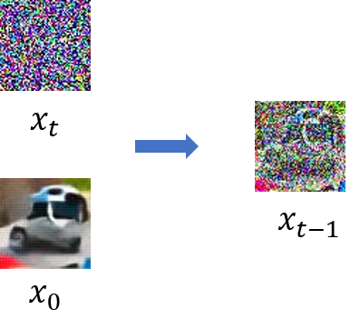
注意$q\left({\mathbf{x}}_t\mid {\mathbf{x}}_{t-1}\right)$是已知量，我们可以使用贝叶斯的方式推导出$q\left({\mathbf{x}}_{t-1}\mid {\mathbf{x}}_t\right)$，作者在这里并没有试图直接表示$q\left({\mathbf{x}}_{t-1}\mid {\mathbf{x}}_t\right)$，而是试图寻找$q\left({\mathbf{x}}_{t-1}\mid {\mathbf{x}}_t,{\mathbf{x}}_0\right)$的表示形式，我们可以从直觉上理解这样表示的原因：
给定一张全部为高斯噪声的$T$时刻的图像，想要预测前一个时刻的图像是很难的：

但是如果同时知道${\mathbf{x}}_t,{\mathbf{x}}_0$，就容易预测前一个时刻的分布：

根据马尔科夫过程的马尔科夫属性，某时刻的状态只与上一个时刻的状态有关，而与之前的无关，我们可以重新表示$q\left({\mathbf{x}}_t\mid {\mathbf{x}}_{t-1}\right)$：
$$q\left({\mathbf{x}}_t\mid {\mathbf{x}}_{t-1}\right)=q\left({\mathbf{x}}_t\mid {\mathbf{x}}_{t-1},{\mathbf{x}}_0\right)$$
我们看一下如果将我们要找的$q\left({\mathbf{x}}_{t-1}\mid {\mathbf{x}}_t,{\mathbf{x}}_0\right)$转到上式，需要经过怎样的变换：
$$\begin{array}{rl}q\left({\mathbf{x}}_{t-1}\mid {\mathbf{x}}_t,{\mathbf{x}}_0\right)& =\frac{q\left({\mathbf{x}}_{t-1},{\mathbf{x}}_t,{\mathbf{x}}_0\right)}{q\left({\mathbf{x}}_t,{\mathbf{x}}_0\right)}\\ & =\frac{q\left({\mathbf{x}}_t\mid {\mathbf{x}}_{t-1},{\mathbf{x}}_0\right)\cdot q\left({\mathbf{x}}_{t-1},{\mathbf{x}}_0\right)}{q\left({\mathbf{x}}_t,{\mathbf{x}}_0\right)}\\ & =\frac{q\left({\mathbf{x}}_t\mid {\mathbf{x}}_{t-1}\right)\cdot q\left({\mathbf{x}}_{t-1},{\mathbf{x}}_0\right)}{q\left({\mathbf{x}}_t,{\mathbf{x}}_0\right)}\\ & =\frac{q\left({\mathbf{x}}_t\mid {\mathbf{x}}_{t-1}\right)\cdot q\left({\mathbf{x}}_{t-1}\mid {\mathbf{x}}_0\right)\cdot q\left({\mathbf{x}}_0\right)}{q\left({\mathbf{x}}_t\mid {\mathbf{x}}_0\right)\cdot q\left({\mathbf{x}}_0\right)}\\ & =\frac{q\left({\mathbf{x}}_t\mid {\mathbf{x}}_{t-1}\right)\cdot q\left({\mathbf{x}}_{t-1}\mid {\mathbf{x}}_0\right)}{q\left({\mathbf{x}}_t\mid {\mathbf{x}}_0\right)}\end{array}$$
因此，重新用$q\left({\mathbf{x}}_{t-1}\mid {\mathbf{x}}_t,{\mathbf{x}}_0\right)$表示$q\left({\mathbf{x}}_t\mid {\mathbf{x}}_{t-1}\right)$：
$$q\left({\mathbf{x}}_t\mid {\mathbf{x}}_{t-1}\right)=\frac{q\left({\mathbf{x}}_{t-1}\mid {\mathbf{x}}_t,{\mathbf{x}}_0\right)q\left({\mathbf{x}}_t\mid {\mathbf{x}}_0\right)}{q\left({\mathbf{x}}_{t-1}\mid {\mathbf{x}}_0\right)}$$
将上面的结果替换到$\log \left(\frac{q\left({\mathbf{x}}_{1:T}\mid {\mathbf{x}}_0\right)}{p_{\theta }\left({\mathbf{x}}_{0:T}\right)}\right)$中：
$$\begin{array}{rl}\log \left(\frac{q\left({\mathbf{x}}_{1:T}\mid {\mathbf{x}}_0\right)}{p_{\theta }\left({\mathbf{x}}_{0:T}\right)}\right)& =-\log \left(p\left({\mathbf{x}}_T\right)\right)+\sum _{t=2}^T\log \frac{q\left({\mathbf{x}}_t\mid {\mathbf{x}}_{t-1}\right)}{p_{\theta }\left({\mathbf{x}}_{t-1}\mid {\mathbf{x}}_t\right)}+\log \frac{q\left({\mathbf{x}}_1\mid {\mathbf{x}}_0\right)}{p_{\theta }\left({\mathbf{x}}_0\mid {\mathbf{x}}_1\right)}\\ & =-\log \left(p\left({\mathbf{x}}_T\right)\right)+\sum _{t=2}^T\log \frac{q\left({\mathbf{x}}_{t-1}\mid {\mathbf{x}}_t,{\mathbf{x}}_0\right)q\left({\mathbf{x}}_t\mid {\mathbf{x}}_0\right)}{p_{\theta }\left({\mathbf{x}}_{t-1}\mid {\mathbf{x}}_t\right)q\left({\mathbf{x}}_{t-1}\mid {\mathbf{x}}_0\right)}+\log \frac{q\left({\mathbf{x}}_1\mid {\mathbf{x}}_0\right)}{p_{\theta }\left({\mathbf{x}}_0\mid {\mathbf{x}}_1\right)}\\ & =-\log \left(p\left({\mathbf{x}}_T\right)\right)+\sum _{t=2}^T\log \left(\frac{q\left({\mathbf{x}}_{t-1}\mid {\mathbf{x}}_t,{\mathbf{x}}_0\right)}{p_{\theta }\left({\mathbf{x}}_{t-1}\mid {\mathbf{x}}_t\right)}\right)+\sum _{t=2}^T\log \left(\frac{q\left({\mathbf{x}}_t\mid {\mathbf{x}}_0\right)}{q\left({\mathbf{x}}_{t-1}\mid {\mathbf{x}}_0\right)}\right)+\log \left(\frac{q\left({\mathbf{x}}_1\mid {\mathbf{x}}_0\right)}{p_{\theta }\left({\mathbf{x}}_0\mid {\mathbf{x}}_1\right)}\right)\end{array}$$
我们先短暂的来看一下为什么最后那一项要单独拿出来：
$$\frac{q\left({\mathbf{x}}_1\mid {\mathbf{x}}_0\right)}{p_{\theta }\left({\mathbf{x}}_0\mid {\mathbf{x}}_1\right)}=\frac{q\left({\mathbf{x}}_0\mid {\mathbf{x}}_1,{\mathbf{x}}_0\right)q\left({\mathbf{x}}_1\mid {\mathbf{x}}_0\right)}{q\left({\mathbf{x}}_0\mid {\mathbf{x}}_0\right)}$$
这里面的$q\left({\mathbf{x}}_0\mid {\mathbf{x}}_1,{\mathbf{x}}_0\right)$和$q\left({\mathbf{x}}_0\mid {\mathbf{x}}_0\right)$没有什么意义，所以单独考虑。接下来，我们将注意力放在中间两项上：
我们将第三项展开，以$T=4$为例：
$$\begin{array}{rl}\sum _{t=2}^4\log \frac{q\left({\mathbf{x}}_t\mid {\mathbf{x}}_0\right)}{q\left({\mathbf{x}}_{t-1}\mid {\mathbf{x}}_0\right)}& =\log \prod _{t=2}^4\frac{q\left({\mathbf{x}}_t\mid {\mathbf{x}}_0\right)}{q\left({\mathbf{x}}_{t-1}\mid {\mathbf{x}}_0\right)}\\ & =\log \frac{q\left({\mathbf{x}}_2\mid {\mathbf{x}}_0\right)q\left({\mathbf{x}}_3\mid {\mathbf{x}}_0\right)q\left({\mathbf{x}}_4\mid {\mathbf{x}}_0\right)}{q\left({\mathbf{x}}_1\mid {\mathbf{x}}_0\right)q\left({\mathbf{x}}_2\mid {\mathbf{x}}_0\right)q\left({\mathbf{x}}_3\mid {\mathbf{x}}_0\right)}\\ & =\log \frac{q\left({\mathbf{x}}_4\mid {\mathbf{x}}_0\right)}{q\left({\mathbf{x}}_1\mid {\mathbf{x}}_0\right)}\end{array}$$
所以这一项实际上是可以化简的，我们再次重写$\log \left(\frac{q\left({\mathbf{x}}_{1:T}\mid {\mathbf{x}}_0\right)}{p_{\theta }\left({\mathbf{x}}_{0:T}\right)}\right)$：
$$\begin{array}{rl}\log \left(\frac{q\left({\mathbf{x}}_{1:T}\mid {\mathbf{x}}_0\right)}{p_{\theta }\left({\mathbf{x}}_{0:T}\right)}\right)& =-\log \left(p\left({\mathbf{x}}_T\right)\right)+\sum _{t=2}^T\log \left(\frac{q\left({\mathbf{x}}_{t-1}\mid {\mathbf{x}}_t,{\mathbf{x}}_0\right)}{p_{\theta }\left({\mathbf{x}}_{t-1}\mid {\mathbf{x}}_t\right)}\right)+\sum _{t=2}^T\log \left(\frac{q\left({\mathbf{x}}_t\mid {\mathbf{x}}_0\right)}{q\left({\mathbf{x}}_{t-1}\mid {\mathbf{x}}_0\right)}\right)+\log \left(\frac{q\left({\mathbf{x}}_1\mid {\mathbf{x}}_0\right)}{p_{\theta }\left({\mathbf{x}}_0\mid {\mathbf{x}}_1\right)}\right)\\ & =-\log \left(p\left({\mathbf{x}}_T\right)\right)+\sum _{t=2}^T\log \left(\frac{q\left({\mathbf{x}}_{t-1}\mid {\mathbf{x}}_t,{\mathbf{x}}_0\right)}{p_{\theta }\left({\mathbf{x}}_{t-1}\mid {\mathbf{x}}_t\right)}\right)+\log \left(\frac{q\left({\mathbf{x}}_T\mid {\mathbf{x}}_0\right)}{q\left({\mathbf{x}}_1\mid {\mathbf{x}}_0\right)}\right)+\log \left(\frac{q\left({\mathbf{x}}_1\mid {\mathbf{x}}_0\right)}{p_{\theta }\left({\mathbf{x}}_0\mid {\mathbf{x}}_1\right)}\right)\\ & =-\log \left(p\left({\mathbf{x}}_T\right)\right)+\sum _{t=2}^T\log \left(\frac{q\left({\mathbf{x}}_{t-1}\mid {\mathbf{x}}_t,{\mathbf{x}}_0\right)}{p_{\theta }\left({\mathbf{x}}_{t-1}\mid {\mathbf{x}}_t\right)}\right)+\log q\left({\mathbf{x}}_T\mid {\mathbf{x}}_0\right)-\log p_{\theta }\left({\mathbf{x}}_0\mid {\mathbf{x}}_1\right)\\ & =\log \left(\frac{q\left({\mathbf{x}}_T\mid {\mathbf{x}}_0\right)}{p\left({\mathbf{x}}_T\right)}\right)+\sum _{t=2}^T\log \left(\frac{q\left({\mathbf{x}}_{t-1}\mid {\mathbf{x}}_t,{\mathbf{x}}_0\right)}{p_{\theta }\left({\mathbf{x}}_{t-1}\mid {\mathbf{x}}_t\right)}\right)-\log \left(p_{\theta }\left({\mathbf{x}}_0\mid {\mathbf{x}}_1\right)\right)\end{array}$$
上式可以改写为与KL散度等价的形式：
$$\begin{array}{rl}\log \left(\frac{q\left({\mathbf{x}}_{1:T}\mid {\mathbf{x}}_0\right)}{p_{\theta }\left({\mathbf{x}}_{0:T}\right)}\right)& =\log \left(\frac{q\left({\mathbf{x}}_T\mid {\mathbf{x}}_0\right)}{p\left({\mathbf{x}}_T\right)}\right)+\sum _{t=2}^T\log \left(\frac{q\left({\mathbf{x}}_{t-1}\mid {\mathbf{x}}_t,{\mathbf{x}}_0\right)}{p_{\theta }\left({\mathbf{x}}_{t-1}\mid {\mathbf{x}}_t\right)}\right)-\log \left(p_{\theta }\left({\mathbf{x}}_0\mid {\mathbf{x}}_1\right)\right)\\ & \equiv D_{KL}\left(q\left({\mathbf{x}}_T\mid {\mathbf{x}}_0\right)\Vert p\left({\mathbf{x}}_T\right)\right)+\sum _{t=2}^T{D}_{KL}\left(q\left({\mathbf{x}}_{t-1}\mid {\mathbf{x}}_t,{\mathbf{x}}_0\right)\Vert p_{\theta }\left({\mathbf{x}}_{t-1}\mid {\mathbf{x}}_t\right)\right)-\log (p_{\theta }\left({\mathbf{x}}_0\mid {\mathbf{x}}_1\right)\end{array}$$
上式的第一项$D_{KL}\left(q\left({\mathbf{x}}_T\mid {\mathbf{x}}_0\right)\Vert p\left(x_T\right)\right)$是常数，并且几乎为零，我们将注意力放在后面带参数的两项，我们先具体地求解出$q\left({\mathbf{x}}_{t-1}\mid {\mathbf{x}}_t,{\mathbf{x}}_0\right)$（三个高斯分布相乘）：
$$\begin{array}{rl}q\left({\mathbf{x}}_{t-1}\mid {\mathbf{x}}_t,{\mathbf{x}}_0\right)& =q\left({\mathbf{x}}_t\mid {\mathbf{x}}_{t-1},{\mathbf{x}}_0\right)\frac{q\left({\mathbf{x}}_{t-1}\mid {\mathbf{x}}_0\right)}{q\left({\mathbf{x}}_t\mid {\mathbf{x}}_0\right)}\\ & \propto \exp \left(-\frac{1}{2}\left(\frac{{\left({\mathbf{x}}_t-\sqrt{{\alpha }_t}{\mathbf{x}}_{t-1}\right)}^2}{{\beta }_t}+\frac{{({\mathbf{x}}_{t-1}-\sqrt{{\bar{\alpha }}_{t-1}}{\mathbf{x}}_0)}^2}{1-{\bar{\alpha }}_{t-1}}-\frac{{\left({\mathbf{x}}_t-\sqrt{{\bar{\alpha }}_t}{\mathbf{x}}_0\right)}^2}{1-{\bar{\alpha }}_t}\right)\right)\\ & =\exp \left(-\frac{1}{2}\left(\frac{{\mathbf{x}}_t^2-2\sqrt{{\alpha }_t}{\mathbf{x}}_t{\mathbf{x}}_{t-1}+{\alpha }_t{\mathbf{x}}_{t-1}^2}{{\beta }_t}+\frac{{\mathbf{x}}_{t-1}^2-2\sqrt{{\bar{\alpha }}_{t-1}}{\mathbf{x}}_0{\mathbf{x}}_{t-1}+{\bar{\alpha }}_{t-1}{\mathbf{x}}_0^2}{1-{\bar{\alpha }}_{t-1}}-\frac{{\left({\mathbf{x}}_t-\sqrt{{\bar{\alpha }}_t}{\mathbf{x}}_0\right)}^2}{1-{\bar{\alpha }}_t}\right)\right)\\ & =\exp \left(-\frac{1}{2}\left(\left(\frac{{\alpha }_t}{{\beta }_t}+\frac{1}{1-{\bar{\alpha }}_{t-1}}\right){\mathbf{x}}_{t-1}^2-\left(\frac{2\sqrt{{\alpha }_t}}{{\beta }_t}{\mathbf{x}}_t+\frac{2\sqrt{{\bar{\alpha }}_{t-1}}}{1-{\bar{\alpha }}_{t-1}}{\mathbf{x}}_0\right){\mathbf{x}}_{t-1}+C\left({\mathbf{x}}_t,{\mathbf{x}}_0\right)\right)\right)\end{array}$$

$C\left({\mathbf{x}}_t,{\mathbf{x}}_0\right)$是与${\mathbf{x}}_{t-1}$无关的常数项，这一项太长了，这里就不写了，感兴趣的话可以自行展开计算一下，现在我们要找的是如何用${\mathbf{x}}_t,{\mathbf{x}}_0$来表示高斯分布${\mathbf{x}}_{t-1}$的均值，所以我们希望能够将上式写成$({\mathbf{x}}_{t-1}-M{)}^2$的形式，同时$M$是用${\mathbf{x}}_t,{\mathbf{x}}_0$表示的，下面直接给出结果
令
$${\tilde{\beta }}_t=1/\left(\frac{{\alpha }_t}{{\beta }_t}+\frac{1}{1-{\bar{\alpha }}_{t-1}}\right)=1/\left(\frac{{\alpha }_t-{\bar{\alpha }}_t+{\beta }_t}{{\beta }_t\left(1-{\bar{\alpha }}_{t-1}\right)}\right)=\frac{1-{\bar{\alpha }}_{t-1}}{1-{\bar{\alpha }}_t}\cdot {\beta }_t$$
将第一项${\mathbf{x}}_{t-1}^2$前面的系数变为1，第二项相应地也除以相同的值：
$$\begin{array}{rl}& \left(\frac{\sqrt{{\alpha }_t}}{{\beta }_t}{\mathbf{x}}_t+\frac{\sqrt{{\bar{\alpha }}_{t-1}}}{1-{\bar{\alpha }}_{t-1}}{\mathbf{x}}_0\right)/\left(\frac{{\alpha }_t}{{\beta }_t}+\frac{1}{1-{\bar{\alpha }}_{t-1}}\right)\\ =& \left(\frac{\sqrt{{\alpha }_t}}{{\beta }_t}{\mathbf{x}}_t+\frac{\sqrt{{\bar{\alpha }}_{t-1}}}{1-{\bar{\alpha }}_{t-1}}{\mathbf{x}}_0\right)\frac{1-{\bar{\alpha }}_{t-1}}{1-{\bar{\alpha }}_t}\cdot {\beta }_t\\ =& \frac{\sqrt{{\alpha }_t}\left(1-{\bar{\alpha }}_{t-1}\right)}{1-{\bar{\alpha }}_t}{\mathbf{x}}_t+\frac{\sqrt{{\bar{\alpha }}_{t-1}}{\beta }_t}{1-{\bar{\alpha }}_t}{\mathbf{x}}_0\end{array}$$
实际上${\left[{\mathbf{x}}_{t-1}-(\frac{\sqrt{{\alpha }_t}\left(1-{\bar{\alpha }}_{t-1}\right)}{1-{\bar{\alpha }}_t}{\mathbf{x}}_t+\frac{\sqrt{{\bar{\alpha }}_{t-1}}{\beta }_t}{1-{\bar{\alpha }}_t}{\mathbf{x}}_0)\right]}^2$的式子展开与上式（每一项都除以$(\frac{{\alpha }_t}{{\beta }_t}+\frac{1}{1-{\bar{\alpha }}_{t-1}}$）一致。好了，现在我们求解得到了$q\left({\mathbf{x}}_{t-1}\mid {\mathbf{x}}_t,{\mathbf{x}}_0\right)$的分布：
$$\begin{array}{rl}q\left({\mathbf{x}}_{t-1}\mid {\mathbf{x}}_t,{\mathbf{x}}_0\right)& =\mathcal{N}\left({\mathbf{x}}_{t-1};\tilde{\mathbf{\mu }}\left({\mathbf{x}}_t,{\mathbf{x}}_0\right),{\tilde{\beta }}_t\mathbf{I}\right)\\ where& \tilde{\mathbf{\mu }}\left({\mathbf{x}}_t,{\mathbf{x}}_0\right)=\frac{\sqrt{{\alpha }_t}\left(1-{\bar{\alpha }}_{t-1}\right)}{1-{\bar{\alpha }}_t}{\mathbf{x}}_t+\frac{\sqrt{{\bar{\alpha }}_{t-1}}{\beta }_t}{1-{\bar{\alpha }}_t}{\mathbf{x}}_0\\ & \tilde{\mathbf{\sigma }}={\tilde{\beta }}_t\end{array}$$
好像在这里看来仍旧没有什么作用，损失函数里面还是有很多的内容，现在我们先来看一下损失函数变成了什么，只看第二项${\sum }_{t=2}^T{D}_{KL}\left(q\left({\mathbf{x}}_{t-1}\mid {\mathbf{x}}_t,{\mathbf{x}}_0\right)\Vert p_{\theta }\left({\mathbf{x}}_{t-1}\mid {\mathbf{x}}_t\right)\right)$：

系统提示我博客字数太多了，要我分成两篇来写，请接着看下一节:diffusion models 扩散模型公式推导，原理分析与代码（二）🧐🧐🧐🧐