机器学习 - 模型评估

最新推荐文章于 2024-07-25 12:32:58 发布

JOEL-T99

最新推荐文章于 2024-07-25 12:32:58 发布

阅读量521

点赞数

分类专栏：机器学习文章标签：机器学习聚类分类回归 scikit-learn

本文链接：https://blog.csdn.net/weixin_47243236/article/details/119861424

版权

机器学习专栏收录该内容

3 篇文章 0 订阅

订阅专栏

模型评估

二分类模型：交叉验证；准确率、召回率、 $F_1$ 、阈值、ROC & AUC

多分类模型：交叉验证；准确率、召回率、 $F_1$

回归模型：均方误差（MSE）、 $R^2$

聚类模型：轮廓系数

评估方法

留出法

留出法（Hold-Out）：直接将数据集划分为两个互斥的集合，分别作为训练集核测试集，训练出模型后用测试集来评估其测试误差。作为对泛化误差的度量

数据集的划分要尽可能数据分布的一致性，避免分布差异造成对结果的影响。单次的留出法得到的结果往往不够可靠，应当采用若干次随机化分、重复进行试验评估后取均值作为留出法的评估结果。

局限性：

若划分的训练集较大，训练模型更接近于原数据集训练的模型，但会因测试集较小，造成评估结果不准确
若划分的测试集较大，训练出的模型与原数据集训练的模型有较大差异，则会降低评估结果的保真性

自助法

自助法（Bootstrapping）：直接以自助采样法为基础，一定程度上降低了数据集规模。

自助法产生的数据集改变了原数据集的分布，会造成估计偏差，当数据集较大时，留出法和交叉验证更常用。

交叉验证法

交叉验证（Cross-Validation）：是一种评估泛化性能的统计学方法。

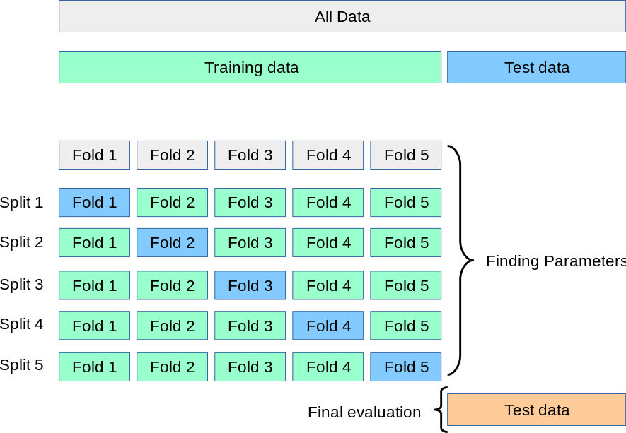
K折交叉验证

K折交叉验证（K-Fold Cross-Validation，KFCV）：数据被划分为k份，将其中k-1份数据作为训练集，另外一份作为测试集，重复训练k次。每次都取不同的训练集，最终将模型在k次迭代中的到的得分取平均值作为总体得分。

from sklearn.model_selection import cross_val_score
from sklearn.linear_model import LogisticRegression
from sklearn.datasets import load_iris

iris = load_iris()

logistic = LogisticRegression()

scores = cross_val_score(logistic, iris.data, iris.target)

score.mean()

'''
OUT:
0.9733333333333334
'''

注：cross_val_score 默认执行3次交叉验证，可以通过设定cv参数来修改折数

K折交叉验证无法处理偏斜数据集以及标签集中排列的数据集，这时可以使用分层K折交叉验证。

分层K折交叉验证

分层K折交叉验证（Stratified K-Fold Cross-Validation）：划分数据，使每个折中类别之间的比例与整个数据集中的比例相同。

import numpy as np
from sklearn.model_selection import StratifiedKFold
X = np.array([[1, 2], [3, 4], [1, 2], [3, 4]])
y = np.array([0, 0, 1, 1])
skf = StratifiedKFold(n_splits=2)
for train_index, test_index in skf.split(X, y):
    print("TRAIN:", train_index, "TEST:", test_index)
    X_train, X_test = X[train_index], X[test_index]
    y_train, y_test = y[train_index], y[test_index]

'''
OUT:
TRAIN: [1 3] TEST: [0 2]
TRAIN: [0 2] TEST: [1 3]
'''

交叉策略

交叉验证分离器

sklearn允许提供一个交叉验证分离器（Cross-Validation Splitter）作为cv参数，cv用于指定使用什么样的交叉验证方法。

from sklearn.model_selection import KFold
kfold = KFold(n_splits=5, shuffle=True, random_state=0)

scores = cross_val_score(logistic, iris.data, iris.target, cv=kfold)
scores.mean()

'''
OUT:
0.9533333333333334
'''

注：shuffle=True：打乱数据

留一法交叉验证

留一法（Leave-One-Out）：提供训练/测试索引以拆分训练/测试集中的数据。每个样本用作测试集（单例）一次，其余样本构成训练集。

from sklearn.model_selection import LeaveOneOut
loo = LeaveOneOut()

scores = cross_val_score(logistic, iris.data, iris.target, cv=loo)
scores.mean()

'''
OUT:
0.9666666666666667
'''

打乱划分交叉验证

打乱划分交叉验证（Shuttle-Split Cross-Validation）：生成索引以将数据拆分为训练集和测试集。

from sklearn.model_selection import ShuffleSplit
shuffle = ShuffleSplit(test_size=.5, train_size=.5, n_splits=10)

scores = cross_val_score(logistic, iris.data, iris.target, cv=shuffle)
scores.mean()

'''
OUT:
0.9560000000000001
'''

打乱划分交叉验证可以设定迭代次数，还有另外一种分层形式名为StratifiedShuffleSplit，可以为分类任务提供更可靠的结果。

分组交叉验证

分组交叉验证（Group Cross-Validation）：同一组不会出现在两个不同的折叠中（不同组的数量必须至少等于折叠的数量）。在每个折叠中不同组的数量大致相同的意义上，折叠是近似平衡的。

import numpy as np
from sklearn.model_selection import GroupKFold
X = np.array([[1, 2], [3, 4], [5, 6], [7, 8]])
y = np.array([1, 2, 3, 4])
groups = np.array([0, 0, 2, 2])
group_kfold = GroupKFold(n_splits=2)

for train_index, test_index in group_kfold.split(X, y, groups):
    print("TRAIN:", train_index, "TEST:", test_index)
    X_train, X_test = X[train_index], X[test_index]
    y_train, y_test = y[train_index], y[test_index]
    
'''
OUT:
TRAIN: [0 1] TEST: [2 3]
TRAIN: [2 3] TEST: [0 1]
'''

性能度量

对于二分类问题的评估，一种最全面的表示方法是使用混淆矩阵。

混淆矩阵

在这里插入图片描述

from sklearn.linear_model import LogisticRegression
from sklearn.model_selection import train_test_split
from sklearn.metrics import confusion_matrix
from sklearn.datasets import load_digits

digits = load_digits()
y = digits.target == 9
X_train, X_test, y_train, y_test = train_test_split(digits.data, y, random_state=0)

logistic = LogisticRegression(C=.1).fit(X_train,y_train)
pre_logistic = logistic.predict(X_test)

confusion = confusion_matrix(y_test, pre_logistic)
print("Condusion = matrix: \n{}".format(confusion))

'''
OUT:
Condusion matrix: 
[[402   1]
 [  6  41]]
'''

精度/错误率

精度： $\frac{TP+TN}{TP+TN+FP+FN}$

错误率： $\frac{FP+FN}{TP+TN+FP+FN}$

查准/查全率

准确（查准）率： 被预测为正例的样本中有多少是真正的正例
$\frac{TP}{TP+FP}$
召回（查全）率： 正类样本中有多少被预测为正类
$\frac{TP}{TP+FN}$

from sklearn.metrics import precision_score, recall_score
P = precision_score(y_test, pre_logistic)
R = recall_score(y_test, pre_logistic)
print(
    "Precision Score: {}".format(P),
    "\nRecall Score: {}".format(R)
)

'''
OUT:
Precision Score: 0.9761904761904762 
Recall Score: 0.8723404255319149
'''

P-R曲线

P-R图可以直观地显示出学习器在样本总体上的查准率与查全率，若一个学习器的曲线（蓝色C）被另一个学习器的曲线（橙色B或黑色A）完全”包住“，则认为后者的性能优于前者。若两个学习器的曲线（橙色B与黑色A）发生了交叉，则需要在具体的查准率或查全率条件下比较，但通常认为一个学习器的P-R曲线的下面积在一定程度上表征了两率取得双高的比例。

import numpy as np
import matplotlib.pyplot as plt
from sklearn.metrics import precision_recall_curve

precision, recall, thresholds = precision_recall_curve(y_test, logistic.predict_proba(X_test)[:,1])
plt.plot(recall,precision)
plt.title('Precision/Recall Curve')
plt.xlabel('Recall Score')
plt.ylabel('Precision Score')
plt.show()

注：输出如下图

在这里插入图片描述

$F_1$ 度量

对准确率和召回率进行综合度量的方法被称为** $F_1$ -分数**（F-Score）或** $F_1$ -度量**（F-Measure），它是调和平均值（一种用于概率数据的平均数）：
$F_1 = 2·\frac{Presiison·Recall}{Presiison+Recall} = \frac{2·TP}{2·TP+FP+FN}$

from sklearn.metrics import f1_score
F1 = f1_score(y_test, pre_logistic)
print("F1 Score: \n{}".format(F1))

'''
OUT:
F1 Score: 
0.9213483146067415
'''

性能报告

from sklearn.metrics import classification_report
print(classification_report(y_test, pre_logistic))

'''
OUT:
              precision    recall  f1-score   support

       False       0.99      1.00      0.99       403
        True       0.98      0.87      0.92        47

    accuracy                           0.98       450
   macro avg       0.98      0.93      0.96       450
weighted avg       0.98      0.98      0.98       450
'''

阈值

阈值（thresholds）：用于权衡准确率与召回率，降低阈值会在增加召回率的同时降低精度。

准确率-召回率曲线（Precision-Recall Curve）：能够计算P-R曲线。precision_recall_curve函数返回一个列表，包含按顺序排列的所有可能的阈值对应的准确率和召回率。这个函数需要真实标签与预测标签的不确定度，由decision_funciton或predict_proba给出

from sklearn.metrics import precision_recall_curve
precision, recall, thresholds = precision_recall_curve(y_test, logistic.predict_proba(X_test)[:,1])

def plot_precision_recall_vs_thresholds(precision, recall, thresholds):
    plt.plot(thresholds, precision[:-1], 'b--', label='Precision')
    plt.plot(thresholds, recall[:-1], 'g-', label='Recall')
    plt.xlabel('Thresholds')
    plt.legend(loc=3)
    plt.ylim([0,1])
    
plot_precision_recall_vs_thresholds(precision, recall, thresholds)
plt.show()

注：输出如下图

在这里插入图片描述

提高阈值可以让去曲线向准确度更高的方向移动，但同时会降低召回率。增大阈值，大多数被划分为正类的点都是真正例（TP）。随着准确率的升高，模型越能够保持较高的召回率，则模型越好。

ROC & AUC

受试者工程特征曲线（Receiver Operating Characteristics Curve，ROC）：是评估二元分类器质量的常用方法，与P-R曲线类似，ROC曲线考虑了给定分类器的所有可能的阈值，但它显示的是假正例率（False Positive Rate，FPR）与真正例率（True Positive Rate，TPR）。FPR、TPR可以使用roc_curve计算。

我们根据学习器预测结果对样例排序，按此顺序逐个把样本作为正例进行预测，每次计算出两个重要量的值，分别以它们为横、纵坐标作图，就得到了ROC曲线。

TPR： $\frac{TP}{TP+FN}$

FPR： $\frac{FP}{TN+FP}$

from sklearn.metrics import roc_curve
fpr, tpr, thresholds = roc_curve(y_test, logistic.predict_proba(X_test)[:,1])

def plot_roc_curve(fpr, tpr, thresholds):
    plt.plot(fpr, tpr, label="ROC Curve")
    plt.plot([0,1], [0,1], 'k--')
    # 找到最接近于0的阈值
    close_zero = np.argmin(thresholds)
    plt.plot(fpr[close_zero], tpr[close_zero], 'o', markersize=10,
            label='thresholds zero', fillstyle='none', c='k', mew=2)
    plt.xlabel('Flase Prositive Rate')
    plt.ylabel('True Prositive Rate')
    plt.legend(loc=4)
    
plot_roc_curve(fpr, tpr, thresholds)
plt.show()

注：输出如下图

在这里插入图片描述

由图可见，TPR（召回率）越高，分类器产生的FPR（假正例）就越多，虚线表示纯随机分类器的ROC曲线，一个优秀的分类器应该离这条线越远越好（左上角）。

ROC / P-R 选择：

当正例非常少见或者更关注假正例而不是假反例时，应该选择PR曲线，反之则是ROC曲线。

与P-R曲线一样，希望有一个指标能综合评价ROC曲线，有一个方法是测量曲线下面积，通常被称为AUC（Area Under The Curve），我们可以利用roc_auc_score函数来计算ROC曲线下的面积。面积较大模型，其性能越好。

from sklearn.metrics import roc_auc_score
roc_auc_score(y_test, pre_logistic)

'''
OUT:
0.9349295179768755
'''

建议在不平衡数据集上评估模型时使用AUC，AUC没有使用默认阈值，因此为了在高AUC的模型中得到有用的分类结果，可能还需要调节决策阈值。

均方误差

均方误差（Mesn Squared Error，MSE）：回归模型最常用的评估指标之一。

$\frac{1}{2}\sum_{i=1}^n(\hat{y}_i-y_i)^2$
其中， $n$ 是样本的数量， $y_i$ 是样本 $i$ 的真实值， $\hat{y}_i$ 是模型对 $y_i$ 的预测值，MSE是预测值和真实值距离的平方和，值越大对应模型性能越差。在sklearn中应该使用 neg_mean_squared_error 参数，它是MSE的像相反数。

$R^2$

决定系数（ $R^2$ ）：代表目标向量的变化中有多少能通过模型进行解释。 $R^2$ 得分越接近1，代表模型性能越好。
$R^2 = 1-\frac{\sum_{i=1}^n(y_i-\hat{y}_i)^2}{\sum_{i=1}^n(y_i-\overline{y})^2}$
其中， $y_i$ 表示样本 $i$ 的真实性， $\hat{y}_i$ 是样本 $y_i$ 的预测值， $\overline{y}$ 是目标向量的平均值。

轮廓系数

轮廓系数（Silhouette Coefficient）：可以用来衡量聚类模型的质量。轮廓系数取值范围为[-1,1]，取值越接近1则说明聚类性能越好，相反，取值越接近-1则说明聚类性能越差，取值为0时说明有簇重叠。

第 $i$ 个样本的轮廓系数的计算公式为：
$s_i = \frac{b_i-a_i}{max(a_i,b_i)}$
其中， $s_i$ 是样本 $i$ 的轮廓系数， $a_i$ 是样本 $i$ 与同类的所有样本间的平均距离， $b_i$ 是样本 $i$ 与来自不同分类的最近聚类的所有样本间的平均距离。

轮廓系数不能作为不同聚类模型间的对比依据，对于簇结构为凸的数据轮廓系数值高，而对于簇结构非凸的数据，轮廓系数值低。

JOEL-T99

关注

0
点赞
踩
6

收藏

觉得还不错? 一键收藏
打赏
0
评论
机器学习 - 模型评估

模型评估二分类模型：交叉验证；准确率、召回率、F1F_1F1、阈值、ROC & AUC多分类模型：交叉验证；准确率、召回率、F1F_1F1回归模型：均方误差（MSE）、R2R^2R2聚类模型：轮廓系数评估方法留出法留出法（Hold-Out）：直接将数据集划分为两个互斥的集合，分别作为训练集核测试集，训练出模型后用测试集来评估其测试误差。作为对泛化误差的度量数据集的划分要尽可能数据分布的一致性，避免分布差异造成对结果的影响。单次的留出法得到的结果往往不够可靠，应当采用若干次随机化分
复制链接

扫一扫