【imbalanced库】documentation

官方文档：imbalanced-learn documentation — Version 0.12.2

Useful links: Binary Installers | Source Repository | Issues & Ideas | Q&A Support

• 1. Introduction
  • 1.1. API’s of imbalanced-learn samplers
  • 1.2. Problem statement regarding imbalanced data sets
• 2. Over-sampling
  • 2.1. A practical guide
    • 2.1.1. Naive random over-sampling
    • 2.1.2. From random over-sampling to SMOTE and ADASYN
    • 2.1.3. Ill-posed examples
    • 2.1.4. SMOTE variants
  • 2.2. Mathematical formulation
    • 2.2.1. Sample generation
    • 2.2.2. Multi-class management
• 3. Under-sampling
  • 3.1. Prototype generation
  • 3.2. Prototype selection
    • 3.2.1. Controlled under-sampling techniques
      • 3.2.1.1. Random under-sampling
      • 3.2.1.2. Mathematical formulation
    • 3.2.2. Cleaning under-sampling techniques
      • 3.2.2.1. Tomek’s links
      • 3.2.2.2. Editing data using nearest neighbours
        • 3.2.2.2.1. Edited nearest neighbours
        • 3.2.2.2.2. Repeated Edited Nearest Neighbours
        • 3.2.2.2.3. All KNN
      • 3.2.2.3. Condensed nearest neighbors
        • 3.2.2.3.1. One Sided Selection
    • 3.2.3. Additional undersampling techniques
      • 3.2.3.1. Instance hardness threshold
• 4. Combination of over- and under-sampling
• 5. Ensemble of samplers
  • 5.1. Classifier including inner balancing samplers
    • 5.1.1. Bagging classifier
    • 5.1.2. Forest of randomized trees
    • 5.1.3. Boosting
• 6. Miscellaneous samplers
  • 6.1. Custom samplers
  • 6.2. Custom generators
    • 6.2.1. TensorFlow generator
    • 6.2.2. Keras generator
• 7. Metrics
  • 7.1. Classification metrics
    • 7.1.1. Sensitivity and specificity metrics
    • 7.1.2. Additional metrics specific to imbalanced datasets
    • 7.1.3. Macro-Averaged Mean Absolute Error (MA-MAE)
    • 7.1.4. Summary of important metrics
  • 7.2. Pairwise metrics
    • 7.2.1. Value Difference Metric
• 8. Common pitfalls and recommended practices
  • 8.1. Data leakage
• 9. Dataset loading utilities
  • 9.1. Imbalanced datasets for benchmark
  • 9.2. Imbalanced generator
• 10. Developer guideline
  • 10.1. Developer utilities
    • 10.1.1. Validation Tools
    • 10.1.2. Deprecation
  • 10.2. Making a release
    • 10.2.1. Major release
    • 10.2.2. Bug fix release
• 11. References

Imbalanced-learn（以 imblearn 的形式导入）是一个开源的 MIT 许可库，依赖于 scikit-learn（以 sklearn 的形式导入），为处理不平衡类的分类提供工具。

1.Introduction

1.1. API’s of imbalanced-learn samplers

可用的采样器遵循 scikit-learn API，使用基本估计器，并通过采样方法添加采样功能：

估计器estimator：基础对象，实现从数据中学习的拟合fit方法：

estimator = obj.fit(data, targets)

重采样器resampler：要对数据集进行重新采样，每个采样器都要实现

data_resampled, targets_resampled = obj.fit_resample(data, targets)

不平衡学习采样器接受与 scikit-learn 相同的输入：

• data:

  • 2-D list,

  • 2-D numpy.ndarray,

  • pandas.DataFrame,

  • scipy.sparse.csr_matrix or scipy.sparse.csc_matrix;

• targets:

  • 1-D numpy.ndarray,

  • pandas.Series.

输出结果类型如下：

• data_resampled:

  • 2-D numpy.ndarray,

  • pandas.DataFrame,

  • scipy.sparse.csr_matrix or scipy.sparse.csc_matrix;

• targets_resampled:

  • 1-D numpy.ndarray,

  • pandas.Series.

pandas输入/输出：

与 scikit-learn 不同，imbalanced-learn 支持 Pandas in/out。因此，提供一个数据帧，也会输出一个数据帧。

sparse稀疏输入：

对于稀疏输入，数据在送入采样器之前会转换为压缩稀疏行表示法（参见scipy.sparse.csr_matrix）。为避免不必要的内存拷贝，建议在上游选择 CSR 表示法。

1.2. Problem statement regarding imbalanced data sets

机器学习算法的学习阶段和后续预测可能会受到不平衡数据集问题的影响。平衡问题与不同类别中样本数量的差异相对应。我们说明了在不同的类平衡水平下训练线性 SVM 分类器的效果。

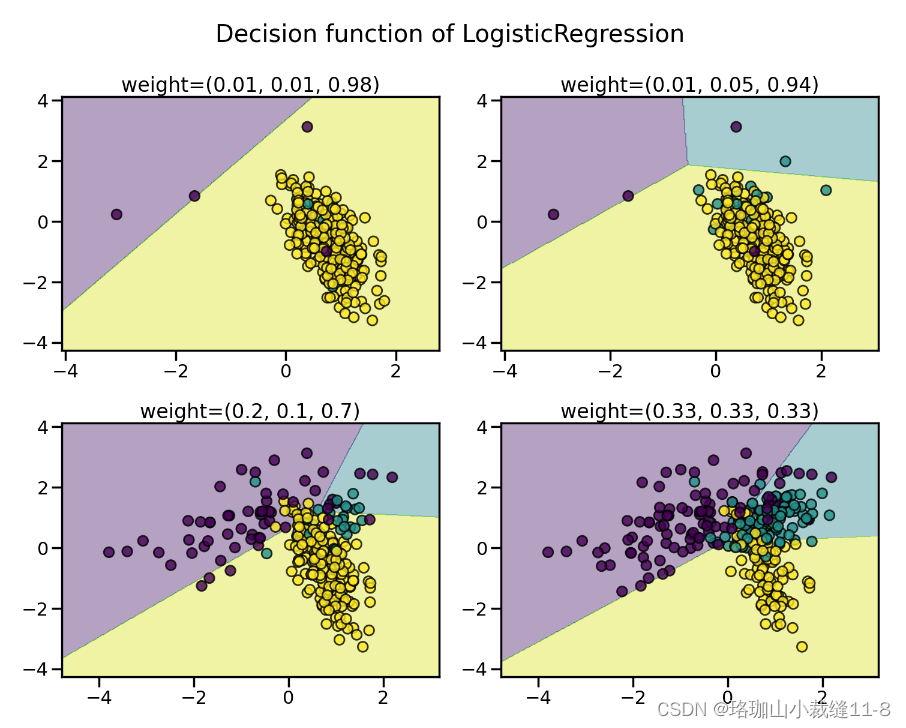
不出所料，线性 SVM 的判定函数会因数据的不平衡程度而有很大不同。不平衡比率越大，决策函数就越倾向于样本数量较多的类，通常称为多数类。

2. Over-sampling

2.1. A practical guide实用指南

您可以参考 Compare over-sampling samplers.

2.1.1. Naive random over-sampling 天真随机过度取样

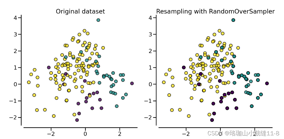
解决这一问题的方法之一是在代表性不足的类别中生成新样本。最简单的方法是对当前可用样本进行随机抽样并替换，从而生成新样本。RandomOverSampler 就提供了这种方案：

from sklearn.datasets import make_classification
X, y = make_classification(n_samples=5000, n_features=2, n_informative=2,
                           n_redundant=0, n_repeated=0, n_classes=3,
                           n_clusters_per_class=1,
                           weights=[0.01, 0.05, 0.94],
                           class_sep=0.8, random_state=0)
from imblearn.over_sampling import RandomOverSampler
ros = RandomOverSampler(random_state=0)
X_resampled, y_resampled = ros.fit_resample(X, y)
from collections import Counter
print(sorted(Counter(y_resampled).items()))

应使用增强数据集代替原始数据集来训练分类器：

from sklearn.linear_model import LogisticRegression
clf = LogisticRegression()
clf.fit(X_resampled, y_resampled)
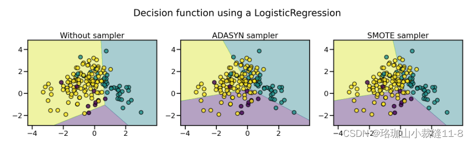
LogisticRegression(...)

在下图中，我们比较了使用过度采样数据集和原始数据集训练的分类器的判定函数。

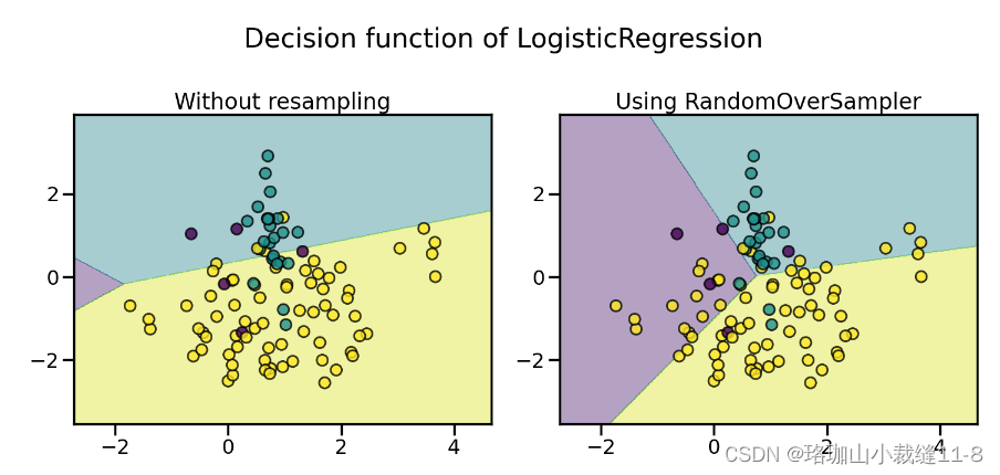
因此，在训练过程中，多数类不会取代其他类。因此，所有类别都能在决策函数中得到体现。

此外，RandomOverSampler 还允许对异构数据（如包含一些字符串）进行采样：

import numpy as np
X_hetero = np.array([['xxx', 1, 1.0], ['yyy', 2, 2.0], ['zzz', 3, 3.0]],
                    dtype=object)
y_hetero = np.array([0, 0, 1])
X_resampled, y_resampled = ros.fit_resample(X_hetero, y_hetero)
print(X_resampled)
print(y_resampled)

它也可以与 pandas 数据帧一起使用：

from sklearn.datasets import fetch_openml
df_adult, y_adult = fetch_openml(
    'adult', version=2, as_frame=True, return_X_y=True)
df_adult.head()  
df_resampled, y_resampled = ros.fit_resample(df_adult, y_adult)
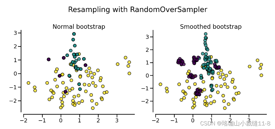
df_resampled.head()  

如果重复样本是一个问题，参数收缩可以创建一个平滑的自举模型。不过，原始数据必须是数值数据。收缩参数可以控制新生成样本的分散性。我们举例说明，使用平滑引导后，新样本不再重叠。这种生成平滑引导的方法也被称为随机过度采样实例（ROSE）[MT14]。

2.1.2. From random over-sampling to SMOTE and ADASYN 从随机过度采样到 SMOTE 和 ADASYN

除了带替换的随机抽样外，还有两种常用的少数群体过度抽样方法：(i) 合成少数群体过度抽样技术（SMOTE）[CBHK02] 和 (ii) 自适应合成（ADASYN）[HBGL08] 抽样方法。这些算法的使用方法相同：

from imblearn.over_sampling import SMOTE, ADASYN
X_resampled, y_resampled = SMOTE().fit_resample(X, y)
print(sorted(Counter(y_resampled).items()))
clf_smote = LogisticRegression().fit(X_resampled, y_resampled)
X_resampled, y_resampled = ADASYN().fit_resample(X, y)
print(sorted(Counter(y_resampled).items()))
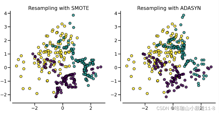
clf_adasyn = LogisticRegression().fit(X_resampled, y_resampled)

下图说明了不同过度取样方法的主要区别。

2.1.3. Ill-posed examples  错综复杂的例子

随机过度采样器（RandomOverSampler）是通过复制少数类的一些原始样本进行过度采样，而 SMOTE 和 ADASYN 则是通过插值生成新样本。不过，用于插值/生成新合成样本的样本有所不同。事实上，ADASYN 的重点是在使用 k 近邻分类器错误分类的原始样本旁边生成样本，而 SMOTE 的基本实现不会区分使用近邻规则分类的易样本和难样本。因此，不同算法在训练过程中找到的判定函数会有所不同。

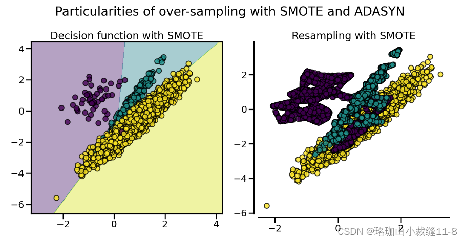
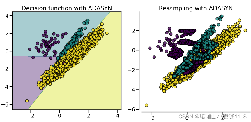
这两种算法的采样特性会导致一些特殊的行为，如下所示。

2.1.4. SMOTE variants  SMOTE 变体

SMOTE 可能会将异常值和异常值联系起来，而 ADASYN 可能只关注异常值，在这两种情况下，都可能会导致决策函数达不到最优。在这方面，SMOTE 提供了另外三种生成样本的方法。这些方法侧重于最优决策函数边界附近的样本，生成的样本方向与最近邻类相反。这些变体如下图所示。

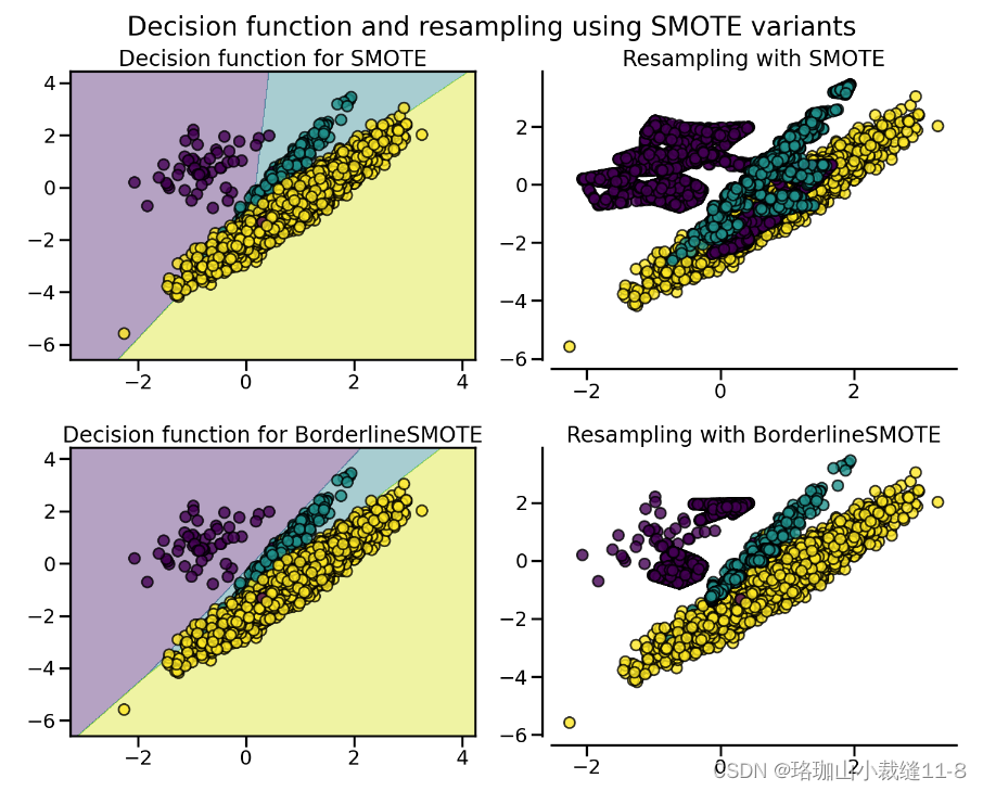
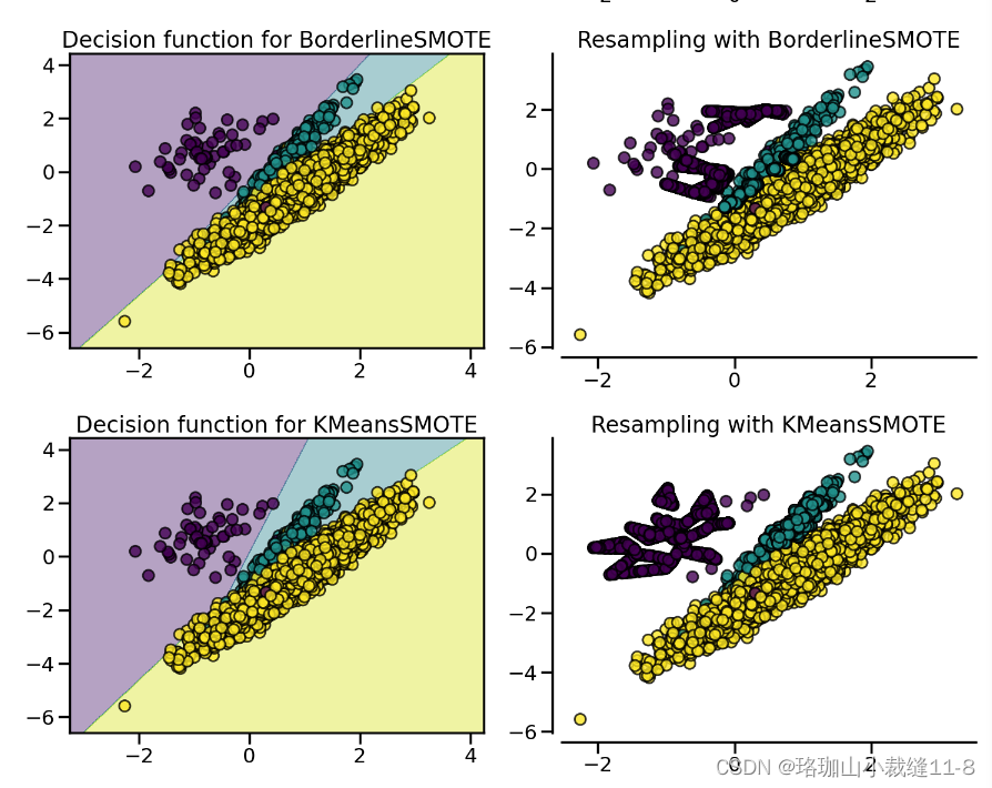
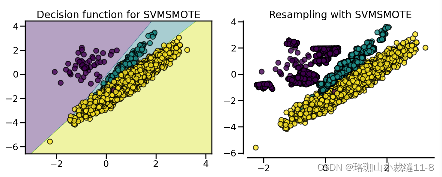BorderlineSMOTE [HWM05]、SVMSMOTE [NCK09] 和 KMeansSMOTE [LDB17] 提供了 SMOTE 算法的某些变体：

from imblearn.over_sampling import BorderlineSMOTE
X_resampled, y_resampled = BorderlineSMOTE().fit_resample(X, y)
print(sorted(Counter(y_resampled).items()))

在处理混合数据类型（如连续特征和分类特征）时，所介绍的方法（除随机过采样器类外）都无法处理分类特征。SMOTENC [CBHK02] 是 SMOTE 算法的一种扩展，它对分类数据进行了不同的处理：

# create a synthetic data set with continuous and categorical features
rng = np.random.RandomState(42)
n_samples = 50
X = np.empty((n_samples, 3), dtype=object)
X[:, 0] = rng.choice(['A', 'B', 'C'], size=n_samples).astype(object)
X[:, 1] = rng.randn(n_samples)
X[:, 2] = rng.randint(3, size=n_samples)
y = np.array([0] * 20 + [1] * 30)
print(sorted(Counter(y).items()))

在这个数据集中，第一个和最后一个特征被视为分类特征。我们需要通过参数 categorical_features 向 SMOTENC 提供这些信息，可以通过传递索引、X 为 pandas DataFrame 时的特征名、标记这些特征的布尔掩码，或者在列使用 pandas.CategoricalDtype 时依靠 dtype 推理：

from imblearn.over_sampling import SMOTENC
smote_nc = SMOTENC(categorical_features=[0, 2], random_state=0)
X_resampled, y_resampled = smote_nc.fit_resample(X, y)
print(sorted(Counter(y_resampled).items()))
print(X_resampled[-5:])

因此，可以看出第一列和最后一列中生成的样本属于最初呈现的相同类别，没有任何其他额外的插值。

不过，SMOTENC 只适用于混合了数字和分类特征的数据。如果数据仅由分类数据组成，则可以使用 SMOTEN 变体 [CBHK02]。该算法有两方面的变化：

1. 近邻搜索并不依赖于欧氏距离。事实上，我们使用的是同样在 ValueDifferenceMetric 类中实现的值差异度量（VDM）。
2. 在生成的新样本中，每个特征值都对应于属于同一类别的邻居样本中最常见的类别。

下面我们来举个例子：

import numpy as np
X = np.array(["green"] * 5 + ["red"] * 10 + ["blue"] * 7,
             dtype=object).reshape(-1, 1)
y = np.array(["apple"] * 5 + ["not apple"] * 3 + ["apple"] * 7 +
             ["not apple"] * 5 + ["apple"] * 2, dtype=object)

我们生成了一个数据集，将一种颜色与是苹果或不是苹果联系起来。我们将 "绿色 "和 "红色 "与苹果紧密联系起来。少数类别是 "非苹果"，我们希望产生的新数据属于 "蓝色 "类别：

from imblearn.over_sampling import SMOTEN
sampler = SMOTEN(random_state=0)
X_res, y_res = sampler.fit_resample(X, y)
X_res[y.size:]
y_res[y.size:]

2.2. Mathematical formulation

2.2.1. Sample generation 样品生成

SMOTE 和 ADASYN 采用相同的算法生成新样本。考虑到样本 xi，则新样本 xnew
 将根据其 k 个近邻（对应于 k_近邻）生成新样本。例如，如下图所示，蓝色圆圈中包括 3 个最近的邻居。然后，从这些近邻中选择一个 xzi 中的一个，并按如下方式生成样本：

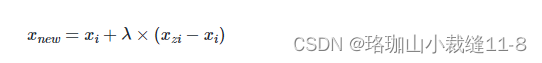
其中 lameda 是在 [0,1]. 该插值法将在 xi 和 xzi 之间的直线上创建样本，如下图所示：

SMOTE-NC 通过对分类特征进行特定处理，稍微改变了生成新样本的方式。事实上，新生成样本的类别是通过挑选生成过程中出现频率最高的近邻类别来决定的。

！！请注意，SMOTE-NC 并非只用于处理分类数据。

SMOTE 的其他变体和 ADASYN 的不同之处在于，在生成新样本之前先选择样本。
 在生成新样本之前选择样本。

常规的 SMOTE 算法（参见 SMOTE 对象）不强加任何规则，而是随机选取所有可能的样本。
 的样本。

边界 SMOTE 算法（参见参数为 kind='borderline-1' 和 kind='borderline-2' 的 BorderlineSMOTE）将对每个样本进行以下分类 xi 

(i) 噪音（即所有近邻都来自不同于 xi的类别不同），(ii) 危险（即至少一半的近邻来自与 
或 (iii)安全（即所有近邻的类别都与 xi). 边界线-1 和边界线-2 SMOTE 将使用危险样本生成新样本。在 Borderline-1 SMOTE 中 xzi 将比样本 xi. 相反，Borderline-2 SMOTE 会考虑 xi 可以来自任何类别。

SVM SMOTE（参照 SVMSMOTE）使用 SVM 分类器查找支持向量，并根据这些支持向量生成样本。请注意，SVM 分类器的 C 参数允许选择更多或更少的支持向量。

对于 borderline 和 SVM SMOTE，都使用参数 m_neighbors 来定义邻域，以决定样本是危险、安全还是噪音。

KMeans SMOTE - 参照 KMeansSMOTE - 在应用 SMOTE 之前使用 KMeans 聚类方法。聚类会将样本集中在一起，并根据聚类密度生成新样本。

ADASYN 的工作原理与普通 SMOTE 类似。不过，每个样本生成的样本数 xi 的样本数量与给定邻域中不属于同一类别的样本数量成正比。xi 的样本数量成正比。因此，在不遵守近邻规则的区域会生成更多样本。参数 m_neighbors 相当于 SMOTE 中的 k_neighbors。

2.2.2. Multi-class management 多类管理

所有算法都可用于多类和二元分类。RandomOverSampler 在样本生成过程中不需要任何类间信息。因此，每个目标类别都是独立重采样的。相反，ADASYN 和 SMOTE 在生成样本时都需要每个样本的邻域信息。它们使用的是一种 "一比一"（one-vs-rest）的方法，即选择每个目标类，并计算与数据集其余部分相对应的必要统计量，而数据集的其余部分被归为一个类。