


Simulink
一、引言:什么是Simulink?
在工程、自动控制、信号处理、电力电子等多个领域中,系统建模和仿真是一项核心技能。而 Simulink,作为 MATLAB 的一个图形化建模与仿真工具,正是实现这一技能的强大利器。
与传统的代码式建模不同,Simulink 提供了一个可视化的拖拽式建模环境,让你像搭积木一样构建复杂的动态系统。无论是从零开始建立一个控制系统,还是将现实系统建模成可仿真的流程,Simulink 都能让你的工作更加直观、快捷、灵活。
Simulink 能做什么?
-
构建动态系统模型(如机械、电气、控制系统等)
-
执行时间域仿真,观察系统响应
-
设计和测试控制器(如 PID 控制)
-
联合 MATLAB 脚本进行数据交互和算法仿真
-
与硬件平台(如 Arduino、Raspberry Pi、实时仿真系统)集成测试
二、安装工作
2.1 安装与初始化
在正式开始搭建模型之前,我们先确保一切准备就绪。本部分将带你完成使用 Simulink 所需的基础准备。Simulink作为 MATLAB 平台上的一个附加工具箱, 要使用它,你需要在安装时勾选 Simulink 工具箱
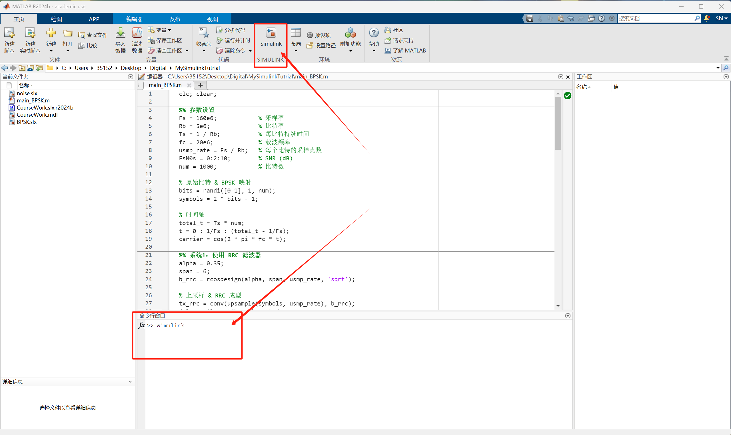
启动 Simulink 有两种常见方式:1、命令行启动:在命令窗口输入 simulink 并回车。2、图标启动:点击 MATLAB 界面上方的 Simulink 图标
2.2 Simulink 界面简介
打开一个新模型后,你会看到:
-
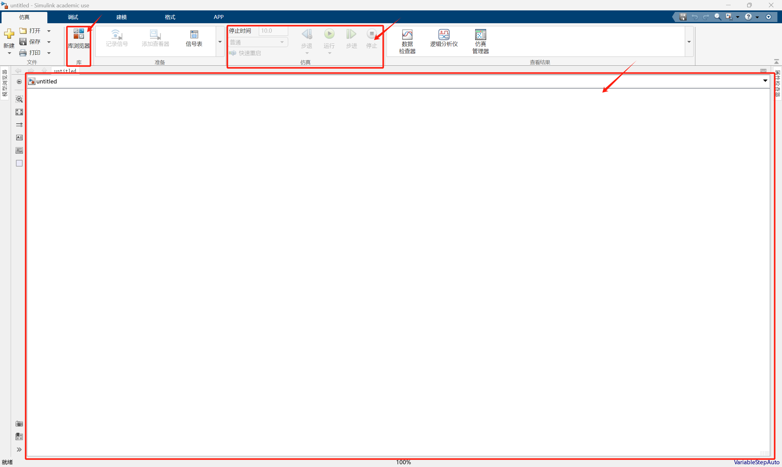
画布(Model Editor): 搭建系统的主工作区
-
库浏览器(Library Browser): 分类展示所有模块(如信号源、运算、逻辑等)
-
工具栏(Toolbar): 包含仿真控制按钮(运行、暂停、停止)和缩放工具
三、构建一个简单仿真
在完成软件环境准备之后,是时候动手建立你的第一个 Simulink 模型了。我们将从一个非常经典的入门示例开始:将一个正弦波信号连接到示波器(Scope)上,观察其波形变化。
这个例子虽然简单,但它涵盖了 Simulink 的基本操作流程:添加模块、连接模块、设置仿真参数、运行模型并查看结果。
3.1 创建新模型
-
打开 MATLAB。
-
输入命令
simulink打开 Simulink 启动页,或点击工具栏上的 Simulink 图标。 -
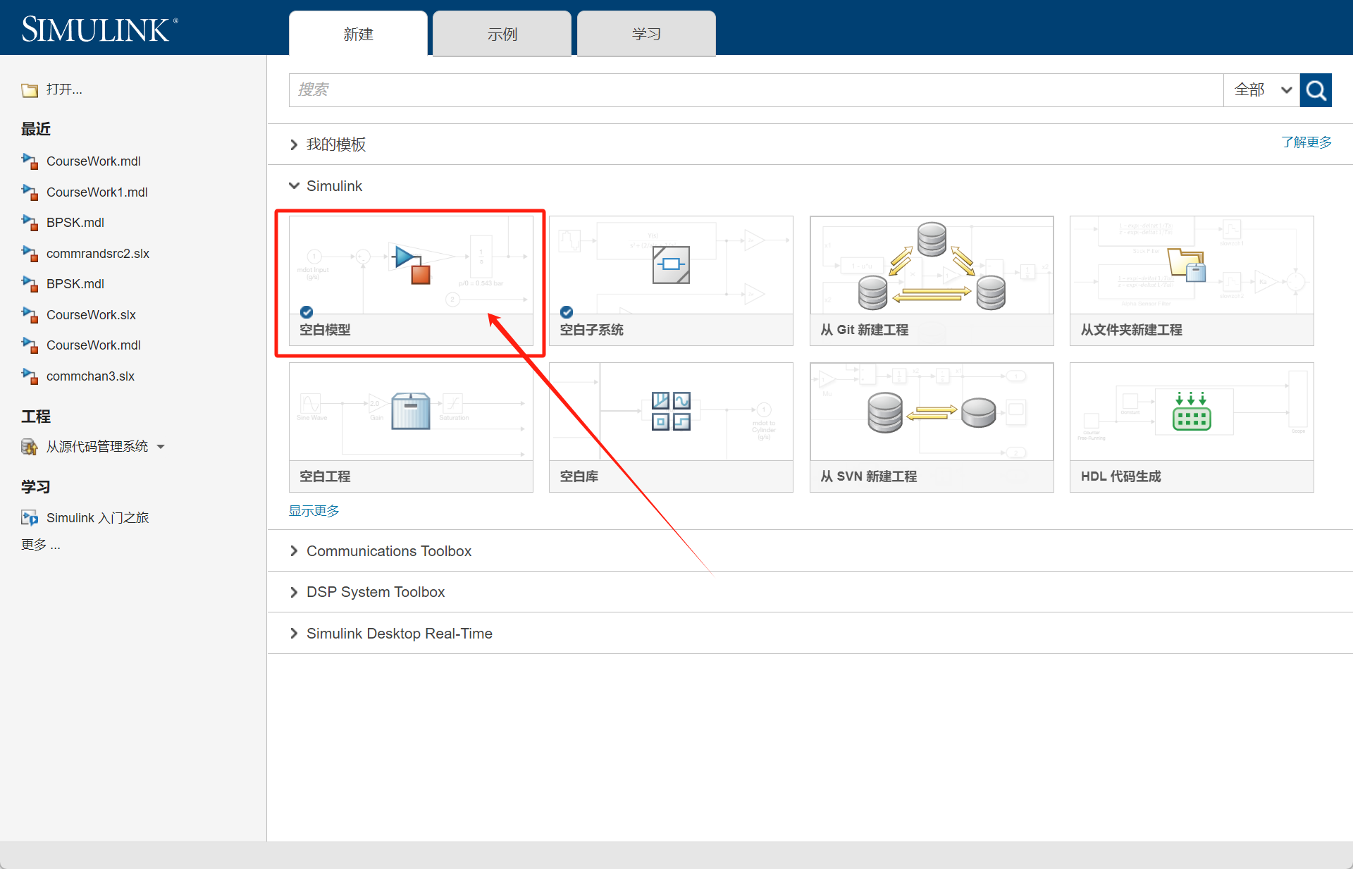
在启动页面点击 空白模型(Blank Model)。
-
会弹出一个新的模型画布界面,点击左上角保存按钮,命名为
first_model.slx。
3.2 添加模块
本模型只需要两个模块:
-
Sine Wave(正弦波):信号源模块
-
Scope(示波器):用于可视化显示信号波形
操作步骤如下:
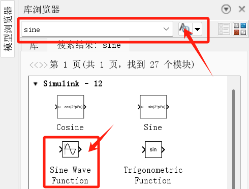
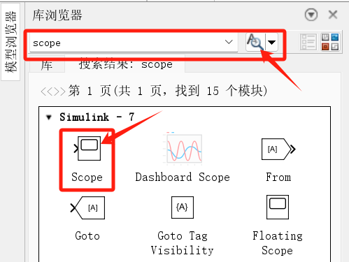
1. 打开 Library Browser(库浏览器)。
2. 在左侧导航栏中:
-
展开 Sources 类别,找到 Sine Wave 模块,拖动到画布(右侧空白区)上;
-
展开 Sinks 类别,找到 Scope 模块,拖动到画布上。
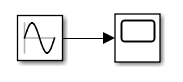
3. 用鼠标将两个模块连接起来:
-
鼠标悬停在 Sine Wave 模块的输出端口(小箭头);
-
拖动连接线至 Scope 模块的输入端口(小箭头),释放即可。
此时你应看到如下结构:
3.3 设置仿真参数
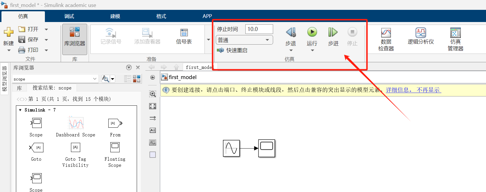
1. 通过仿真区设置参数,若是早期版本没有此区:
-
点击工具栏上的 模型设置(Model Settings),齿轮图标。
-
在弹出的窗口中,点击左侧的 Solver 选项卡。
2. 将 Stop Time(停止时间) 设置为 10.0 秒。
3. 点击 OK(确定) 保存设置。
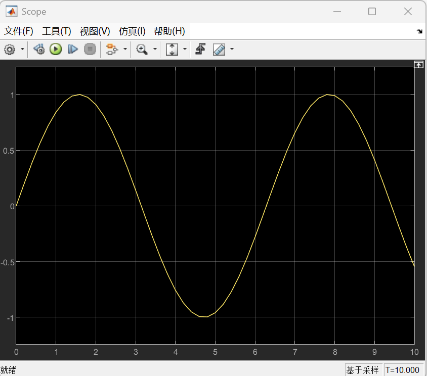
3.4 运行仿真并查看结果
-
点击工具栏中的绿色 运行(Run)按钮。
-
仿真开始后,双击 Scope 模块。
-
你将看到一个动态更新的正弦波图像,横轴为时间,纵轴为幅值。
四、常用模块讲解
Simulink 提供了大量模块,用于构建各种类型的系统。掌握常用模块的作用和用法,是建立复杂模型的前提。
本节将从几个最常用、最基础的模块开始介绍,分为以下几类:
4.1 Sources(信号源)
这类模块用于“产生信号”,作为系统输入,常用于测试系统响应或驱动控制器。
常用模块:
| 模块名 | 功能简介 |
|---|---|
| Sine Wave | 产生连续的正弦波信号,可设置频率、幅度、相位 |
| Step | 产生阶跃信号(如 0→1 的跳变),常用于测试系统响应 |
| Pulse Generator | 产生脉冲信号,可设定周期、占空比 |
| Constant | 输出恒定值 |
| Ramp | 输出线性上升信号 |
4.2 Sinks(输出显示)
Sinks 模块是“结果展示”的窗口,显示信号输出或者保存数据。
常用模块:
| 模块名 | 功能简介 |
|---|---|
| Scope | 示波器,用于显示信号随时间变化的波形 |
| Display | 以数值方式显示信号当前值 |
| To Workspace | 将信号数据导出至 MATLAB 工作区,用于后续绘图或处理 |
| XY Graph | 绘制 X-Y 关系图,用于分析非时间依赖的输入输出关系 |
4.3 Math Operations(数学运算)
用于对信号进行加、减、乘、除等数学处理,是构建控制器和信号处理系统的核心工具。
常用模块:
| 模块名 | 功能简介 |
|---|---|
| Gain | 乘以一个系数(增益) |
| Sum | 加减法运算(可多输入) |
| Product | 乘法(可矩阵或标量) |
| Math Function | 提供如 sin、cos、sqrt 等数学函数操作 |
| Abs | 取绝对值 |
| MinMax | 输出多路输入中的最大或最小值 |
4.4 Continuous / Discrete(连续 / 离散系统)
这些模块用于模拟动态系统,如积分器、传递函数、差分等。
常用模块:
| 模块名 | 功能简介 |
|---|---|
| Integrator | 实现连续时间积分运算 |
| Transfer Function | 定义系统的传递函数模型 |
| Zero-Order Hold | 离散化模拟中用于保持采样值 |
| Discrete-Time Integrator | 离散时间积分器 |
| Unit Delay | 单位时间延迟,用于构建时序逻辑 |
4.5 Logic and Bit Operations(逻辑与位运算)
这些模块用于实现控制逻辑、条件判断、布尔运算等。
常用模块:
| 模块名 | 功能简介 |
|---|---|
| Switch | 条件选择器(如果 A>阈值,则输出 A,否则输出 B) |
| Compare To Constant | 比较输入是否等于、>、< 某个常数 |
| Relational Operator | 输入之间的关系判断,如 A > B |
| Logical Operator | 实现 AND、OR、NOT 等逻辑运算 |
模块命名技巧
模块名称可以重命名,使模型更清晰可读:
-
选中模块 → 右键 → Rename
-
例:将 “Gain” 改名为 “速度控制器增益”,让逻辑更清晰
总结
通过本文的学习,我们从零基础逐步走进了 Simulink 的建模世界。你了解了 Simulink 的定位与主要应用场景,掌握了软件的安装与启动方式,亲手搭建并运行了一个简单的正弦波仿真模型,同时也初步认识了常用模块的功能与使用方法。这些基础内容虽然简单,但却构成了日后构建复杂系统模型的核心基础。Simulink 的优势在于它将抽象的动态系统以可视化的方式呈现,使建模、仿真与调试过程更加直观和高效。未来你可以在此基础上继续深入,尝试构建反馈控制系统、导出仿真数据进行分析,甚至探索与 Stateflow、Simscape 等工具的联合使用。掌握 Simulink,不仅是提升工程建模能力的有力工具,更是打开系统思维与工程实践大门的重要一步。希望本文能为你打下坚实的起点,带来后续学习的信心与方向。
English Version
I. Introduction: What is Simulink?
In fields like engineering, automatic control, signal processing, and power electronics, system modeling and simulation are core skills. Simulink, a graphical modeling and simulation tool within MATLAB, is a powerful platform for mastering these skills.
Unlike traditional code-based modeling, Simulink offers a visual, drag-and-drop environment that lets you build complex dynamic systems as if you were assembling building blocks. Whether you're designing a control system from scratch or modeling a real-world system into a simulatable process, Simulink makes the process more intuitive, efficient, and flexible.
What Can Simulink Do?
-
Model dynamic systems (mechanical, electrical, hydraulic, etc.)
-
Simulate system responses over time
-
Design and test control algorithms (like PID controllers)
-
Integrate with MATLAB scripts for hybrid modeling
-
Interface with hardware (e.g., Arduino, Raspberry Pi, real-time simulators)
II. Installation
2.1 Installing and Initializing
Before we begin building models, let’s make sure everything is set up properly. This section will guide you through the basic preparations required to use Simulink.
Simulink is an add-on toolbox in the MATLAB platform. To use it, make sure to select the Simulink toolbox during installation.
There are two common ways to launch Simulink:
-
Command Line: Type
simulinkin the MATLAB command window and press Enter. -
Toolbar Icon: Click the Simulink icon on the MATLAB toolbar.
2.2 Simulink Interface Overview
After opening a new model, you’ll see the Simulink interface, which includes:
-
Model Editor (Canvas): The main workspace used to build and organize the system model.
-
Library Browser: A categorized view of all available blocks (e.g., signal sources, mathematical operations, logic elements, etc.).
-
Toolbar: Contains simulation control buttons (Run, Pause, Stop) as well as zoom tools.
III. Building a Simple Simulation
With the software environment ready, it's time to build your first Simulink model. We'll start with a classic beginner example: connecting a sine wave signal to a scope to observe waveform changes.
Though simple, this example covers the essential steps in Simulink: adding blocks, connecting them, setting simulation parameters, running the model, and viewing results.
3.1 Creating a New Model
-
Open MATLAB.
-
Type the command
simulinkin the Command Window to open the Simulink Start Page, or click the Simulink icon on the toolbar. -
On the Start Page, click Blank Model to create a new model.
-
A new model canvas window will appear. Click the Save button in the top-left corner, and save the model as first_model.slx.
3.2 Adding Blocks
This model only requires two blocks:
-
Sine Wave (Signal Source): A signal source block that generates a sinusoidal waveform.
-
Scope (Oscilloscope): A visualization block used to display the waveform of the signal in real time.
Steps:
1. Open the Library Browser.
2. In the left-hand navigation panel:
3. Drag and connect the two blocks using your mouse.
You should now see a structure similar to this:
3.3 Setting Simulation Parameters
1. Use the simulation panel to configure parameters. For older versions, use the menu bar.
-
Expand the Sources category in the Library Browser, locate the Sine Wave block, and drag it onto the canvas (the blank area on the right side).
-
Expand the Sinks category, find the Scope block, and drag it onto the canvas as well.
2. Set Stop Time to 10.0 seconds.
3. Click OK to save your settings.
3.4 Running the Simulation and Viewing Results
IV. Commonly Used Blocks
Simulink provides a wide range of blocks for building various types of systems. Understanding the functionality of common blocks is essential for constructing more complex models.
This section introduces frequently used and foundational blocks, categorized as follows:
4.1 Sources
These blocks generate signals to serve as system inputs—ideal for testing system responses or driving controllers.
| Block Name | Description |
|---|---|
| Sine Wave | Generates a continuous sine wave; parameters include frequency, amplitude, phase |
| Step | Generates a step change signal (e.g., 0→1), used to test system response |
| Pulse Generator | Generates pulses with adjustable period and duty cycle |
| Constant | Outputs a constant value |
| Ramp | Outputs a linearly increasing signal |
4.2 Sinks
Sinks display or log output results for analysis.
| Block Name | Description |
|---|---|
| Scope | Oscilloscope for displaying time-varying waveforms |
| Display | Shows the current numerical value of a signal |
| To Workspace | Exports signal data to the MATLAB workspace for plotting or processing |
| XY Graph | Plots X-Y relationships for non-time-dependent input/output analysis |
4.3 Math Operations
Used for mathematical manipulation of signals—crucial for control and signal processing systems.
| Block Name | Description |
|---|---|
| Gain | Multiplies signal by a coefficient |
| Sum | Performs addition or subtraction |
| Product | Performs multiplication (scalar or matrix) |
| Math Function | Includes functions like sin, cos, sqrt, etc. |
| Abs | Computes absolute value |
| MinMax | Outputs the minimum or maximum of multiple inputs |
4.4 Continuous / Discrete
These blocks simulate dynamic systems like integrators, transfer functions, and discrete operations.
| Block Name | Description |
|---|---|
| Integrator | Performs continuous-time integration |
| Transfer Function | Defines system transfer function |
| Zero-Order Hold | Holds sample value for discrete simulation |
| Discrete-Time Integrator | Performs discrete-time integration |
| Unit Delay | Adds one time-step delay, used in sequential logic |
4.5 Logic and Bit Operations
Used for implementing control logic, condition checking, and Boolean operations.
| Block Name | Description |
|---|---|
| Switch | Conditional selector (e.g., output A if A > threshold, else B) |
| Compare To Constant | Compares input to a fixed constant (e.g., ==, >, <) |
| Relational Operator | Compares two inputs (e.g., A > B) |
| Logical Operator | Implements logical operations like AND, OR, NOT |
Block Naming Tip
Block names can be renamed to improve model clarity and readability.
Summary
Through this guide, you’ve stepped into the world of Simulink modeling from the ground up. You’ve learned what Simulink is, how to install and launch it, built and ran your first simple sine wave simulation, and gained an understanding of frequently used blocks and their functions.
These fundamentals may seem simple but form the essential foundation for building complex system models. Simulink's strength lies in its ability to visually represent dynamic systems, making the processes of modeling, simulating, and debugging more intuitive and efficient.
Moving forward, you can build upon this foundation to develop feedback control systems, export simulation data for analysis, and explore integration with tools like Stateflow and Simscape. Mastering Simulink not only enhances your engineering modeling capabilities but also opens the door to systems thinking and practical engineering applications.
May this article be a solid starting point for your journey, providing both confidence and direction for your future learning.


 2万+
2万+

 被折叠的 条评论
为什么被折叠?
被折叠的 条评论
为什么被折叠?
 到【灌水乐园】发言


