Identification of Novel Classes for Improving Few-Shot Object Detection

baseline：FSCE、Detectron、微调 、CVPR，

Abstract

An unexplored challenge for FSOD is that instances from unlabeled novel classes that do not belong to the fixed set of training classes appear in the background.
FSOD面临的一个未探索的挑战是，来自未标记的新类别的实例出现在背景中，这些实例不属于固定的训练类别集合。

Specifically, we propose a hierarchical ternary classification region proposal network (HTRPN) to localize the potential unlabeled novel objects and assign them new objectness labels. Our improved hierarchical sampling strategy for the region proposal network (RPN) also boosts the perception ability of the object detection model for large objects.
我们具体提出了一种分层三元分类区域建议网络（HTRPN），用于定位潜在的未标记的新对象，并为它们分配新的对象性标签。我们改进的区域建议网络（RPN）的分层采样策略还增强了目标检测模型对大型对象的感知能力。

1 Introduction

We study the phenomenon that unlabeled novel object classes that do not belong to either of the base or the labeled novel classes can appear in the training data. For example, we see in Figure. 1 that among base-class training samples, there are a number of objects that remain unlabeled, such as the cow in the image. These unlabeled objects can potentially belong to unseen novel classes. Our experiments demonstrate that this phenomenon exists in PASCAL VOC [4] and COCO [21] datasets。This phenomenon leads to the objectness inconsistency for the model whenarXiv:2303.10422v1 [cs.CV] 18 Mar 2023 recognizing the novel objects: for the novel class, objects are treated as background if their annotations are missing, but they are treated as foreground where they are labeled. Such nonconformity of foreground and background confuses the model when training the objectness and make the model hard to converge and degrades detection accuracy.

3 Problem Descripetion

We formulate the problem of FSOD following a standard setting in the literature [13, 35]. We use the Faster R-CNN network as the object detection model and follow the same evaluation paradigm defined by [35]. Accordingly, the base classes are those classes for which we have sufficient images and instances for each base class (CB ), while novel classes are those for which, we only have a few training samples in the dataset (CN ), where CB ∩ CN = ∅. An n-shot learning scenario means that we have access ton images per seen novel categories. During the pre-training stage, the model is trained only on base class CB , and also is only evaluated on the test set of CB . We then proceed to learn the seen novel classes in the second stage. To overcome catastrophic forgetting about the learned knowledge about the base classes, the pre-trained model is then fine-tuned on both the seen novel classes and base classesCN ∪ CB and then is tested on both sets of classes.
我们按照文献中的标准设置[13, 35]来制定FSOD的问题。我们使用Faster R-CNN网络作为目标检测模型，并按照[35]定义的相同评估范式进行评估。因此，基础类别是那些我们有足够图像和实例的类别（CB），而新颖类别是那些我们在数据集中只有少量训练样本的类别（CN），其中CB ∩ CN = ∅。一个n-shot学习场景意味着我们对每个已见新颖类别有访问n张图像。在预训练阶段，模型仅在基础类别CB上进行训练，并且仅在CB的测试集上进行评估。然后我们继续学习已见新颖类别的第二阶段。为了克服对基础类别学习的知识的灾难性遗忘，预训练模型随后在已见新颖类别和基础类别CN ∪ CB上进行微调，然后在这两个类别集合上进行测试。

Architectures based on R-CNN have been used consistently for object detection. In our work, we improve the R-CNN architecture to identify novel unseen classes as instances that do not belong to the seen classes. For an input image, R-CNN derives five scaled feature maps (p2 ∼ p6) using its feature pyramid network (FPN), and then sizefixed anchors in the region proposal network (RPN) are applied on these feature maps to predict the objectness (i.e.,obj{objpre, objgt, ioua gt}, where objpre is the predicted objectness score in the range of 0 and 1. Here, the ground truth value objgt = 0 indicates a non-object and objgt = 1represents a true object, and ioua gt represents the intersection over the union of an anchor with its ground truth box) and the coarse bounding box (i.e., bboxc) of each anchor to get proposal boxes (i.e., P rop{obj, bboxc, ioup gt}, ioup gtrepresents the intersection over the union of a proposal box with its ground truth box). Anchors with ioua gt > 0.7 are called active anchors (Aa) and their corresponding proposals are called positive proposals (P ropp); while anchors with ioua gt < 0.3 are called negative anchors (An) and the corresponding proposals are called negative proposals (P ropn). Next, P ropp and P ropn are sent to the region of interest pooling layer (RoI pooling) to predict their instance level classification (i.e., clsi, where i is the classification index) and the refined bounding box (i.e., bboxr ). The objects (Obj{clsi, bboxr }) are then finally detected.
基于R-CNN的架构一直被一致地用于目标检测。在我们的工作中，我们改进了R-CNN架构，以识别不属于已见类别的新颖未见类别实例。对于输入图像，R-CNN使用其特征金字塔网络（FPN）推导出五个经过缩放的特征图（p2∼p6），然后在这些特征图上应用尺寸固定的锚点区域建议网络（RPN）来预测目标性（即 o b j { o b j p r e , o b j g t , i o u g t a } obj\{obj_{pre},obj_{gt},iou_{gt}^{a}\} obj{objpre​,objgt​,iougta​}，其中$ob{j}_{pre}$是预测的目标性分数，范围在0到1之间。这里，真实值$ob{j}_{gt}=0$表示非对象，$ob{j}_{gt}=1$表示真实对象，而 $io{u}_{gt}^a$表示锚点与其真实框的交并比），以及每个锚点的粗略边界框（即$bbo{x}_c$），以获得提议框（即 P r o p { o b j , b b o x c , i o u q t p } Prop\{obj,bbox_{c},iou_{qt}^{p}\} Prop{obj,bboxc​,iouqtp​}， $io{u}_{gt}^p$表示提议框与其真实框的交并比）。具有$io{u}_{gt}^a$ > 0.7的锚点被称为活动锚点（Aa），它们对应的提议被称为正提议（$(Pro{p}_p)$）；而具有$io{u}_{gt}^a$< 0.3的锚点被称为负锚点（An），对应的提议被称为负提议（$(Pro{p}_n)$）。接下来，$(Pro{p}_p)$和$(Pro{p}_n)$被送入感兴趣区域池化层（RoI pooling）以预测它们的实例级别分类（即 $cl{s}^i$,其中i是分类索引）和精炼的边界框（即$bbo{x}_r$）。然后最终检测到对象（Obj{$cl{s}^i$，$bbo{x}_r$}）。

The challenge that we want to address stems from the fact that an instance from the unlabeled and unseen novel object (CN pn) can appear in the training dataset in the background (see Figure 2). The reason is that there are many potential classes that we have not included in either the base classes or the unseen novel classes. When detected, these objects would be treated as P ropn and with its ground truth objectness objgtpn = 0. On the contrary, they would be treated as P ropp with ground truth objectness objgtpn = 1if it is labeled as such by the model. These instances can significantly confuse the model when adapting the model for learning the novel unseen classes. We argue that if the unlabeled potential novel object can be distinguished from the P ropn, then its objectness could be modified as a foreground object. Consequently, the inconsistency of the objectness would be eliminated. In other words, we propose to reduce an effect similar to noisy labels as these objects would be objects with wrong labels, leading to confusion in the model and performance degradation.
我们要解决的挑战源于一个事实：未标记和未见的新颖对象（${C_N}^{pn}$）的实例可能出现在训练数据集的背景中（见图2）。原因是我们没有包括在基础类别或未见新颖类别中的许多潜在类别。当检测到时，这些对象将被视为$Pro{p}_n$，并且其真实对象性$ob{j}_{gt}{}^{pn}=0.$。相反，如果模型将其标记为这样的对象，则它们将被视为$Pro{p}_p$，并且其地面实况对象性$ob{j}_{gt}{}^{pn}=1.$。这些实例在调整模型以学习新的未见类别时可能会显著地使模型混淆。我们认为，如果可以将未标记的潜在新颖对象与$Pro{p}_n$区分开来，那么其对象性可以被修改为前景对象。因此，对象性的不一致性将被消除。换句话说，我们建议减少类似于噪声标签的影响，因为这些对象将成为具有错误标签的对象，从而导致模型混淆和性能下降。

Proposed solution

We first demonstrate that it is possible to encounter instances of novel unseen classes during the training stage. We then investigate the relationship between the number of anchors and the size of objects in each feature layer and provide a more effective sampling method for object detection. Finally, we describe our proposed pipeline to pick up objects from unseen classes with high confidence and then explain how we can modify their objectness loss to reduce their adverse effect.
我们首先证明在训练阶段可能会遇到来自新颖未见类别的实例。然后，我们调查了每个特征层中锚点数量与对象大小之间的关系，并提供了一种更有效的目标检测采样方法。最后，我们描述了我们提出的流程，从未见类别中选择具有高置信度的对象，然后解释了如何修改它们的对象性损失以减少它们的不良影响。

4.1. Finding the Potential Proposals

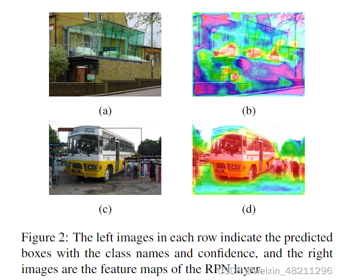
According to the original Faster R-CNN network [28], the unlabeled area in an image would be wrongly treated as background objects in the RPN layer during training. Therefore, the potential unlabeled objects from unseen novel classes are suppressed and hard to be identified as true objects. However, to correct the objectness of these potential objects, the first step is how to find them. We have observed the fact that the network often has clear attention to the potential objects in the RPN layer. As an example, we have used Grad-CAM visualization of the feature map of the RPN layer on some representative training images, as shown in Figure. 2. We observe that although unlabelled novel objects appear in the base training images, the RPN layer could still have strong attention to them, and consequently predict some of them as a known class. In Figure. 2a and 2b, the feature map of p3 layer clearly shows the attention of the “chair” (base class) and “sofa” (novel class), but the sofa is predicted to be an instance of the base class “car”. Similarly, in Figure. 2c and 2d, the potential novel objects (“bus”) can also be seen in the feature map of p4layer, and the “bus” is predicted as an instance of the base class “train”. This observation serves as an inspiration to identify potential proposals: some novel objects have high possibilities to be predicted as known base class.
根据原始的Faster R-CNN网络[28]，图像中的未标记区域在训练过程中会被错误地视为背景对象，在RPN层中被抑制，因此来自未见新颖类别的潜在未标记对象很难被识别为真实对象。然而，要纠正这些潜在对象的对象性，第一步是如何找到它们。我们观察到网络在RPN层对潜在对象通常具有明确的关注。例如，我们对一些代表性的训练图像的RPN层特征图进行了Grad-CAM可视化，如图2所示。我们观察到，虽然未标记的新颖对象出现在基础训练图像中，但RPN层仍然对它们有很强的关注，并因此将其中一些预测为已知类别。在图2a和2b中，p3层的特征图清楚地显示了对“椅子”（基础类别）和“沙发”（新颖类别）的关注，但沙发被预测为基础类别“汽车”的实例。类似地，在图2c和2d中，潜在的新颖对象（“公交车”）也可以在p4层的特征图中看到，并且“公交车”被预测为基础类别“火车”的实例。这一观察为识别潜在提议提供了启示：一些新颖对象很可能被预测为已知的基础类别。

Potential novel unseen class objects that appear in the base class training images usually have lower ioua gt [20] and therefore must be contained by negative anchors (An). Theoretically, there are always exists anchors that can include the potential novel objects in an image. According to the architecture of the RPN layer, anchor boxes are used to determine whether an area contains objects, and each pixel of the feature map will have 3 fixed anchors that are in different sizes and aspect ratios, as shown in Figure. 3a. Consequently, the overall number of anchors decreases for higher feature maps. In the original RPN layer, different sizes of anchors are applied according to the size of the p2to p6 feature maps. Large anchors are more suitable for detecting large objects in high feature layers due to having a larger receptive field, and vice versa. Based on this inch-byinch sliding window liked search, there should exist a sufficient number of candidates An such that they contain potential unseen novel objects. However, to improve the training speed, not all of the anchors are used for determining proposal boxes. For an image, only 256 Aa and An anchors among all feature maps are randomly chosen to participate in the RoI pooling. Nonetheless, this random selection process dramatically reduces the chance to get desired negative anchors for large objects in higher feature maps in terms of probability, since the anchors of large size in p4 to p6 layers intrinsically have fewer cardinal numbers.
通常，出现在基础类别训练图像中的潜在未见类别对象通常具有较低的$io{u}_{gt}^a$[20]，因此必须包含在负锚点（An）中。从理论上讲，在图像中总是存在能够包含潜在新颖对象的锚点。根据RPN层的架构，锚框用于确定一个区域是否包含对象，每个特征图的像素都有3个固定大小和长宽比不同的锚框，如图3a所示。因此，随着特征图尺寸的增加，锚点的总数会减少。在原始的RPN层中，根据p2到p6特征图的大小应用不同尺寸的锚点。由于具有更大的感受野，较大的锚点更适合于在高特征层中检测大型对象，反之亦然。基于这种逐像素滑动窗口式搜索，应该存在足够数量的候选An，这些锚点包含潜在的未见新颖对象。然而，为了提高训练速度，不是所有的锚点都用于确定提议框。对于一个图像，所有特征图中只有256个Aa和An锚点被随机选择参与RoI池化。然而，这个随机选择过程在概率上大大降低了在高特征图中获取所需大型对象的理想负锚点的机会，因为p4到p6层中的大尺寸锚点本质上具有较少的基数。

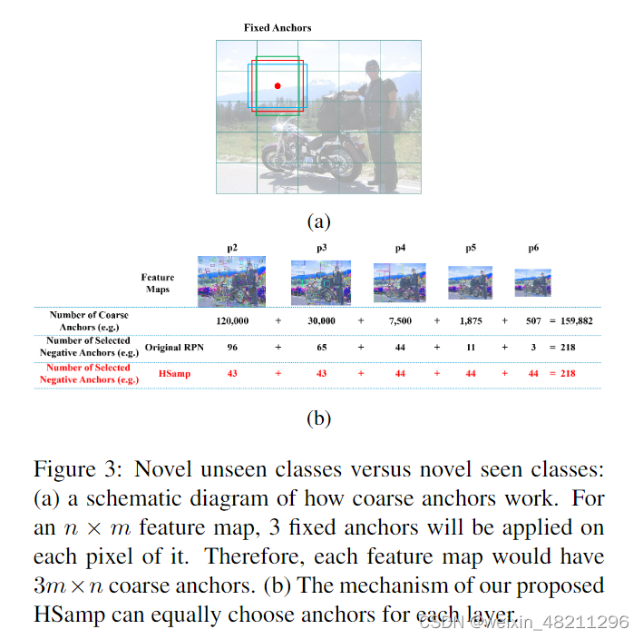
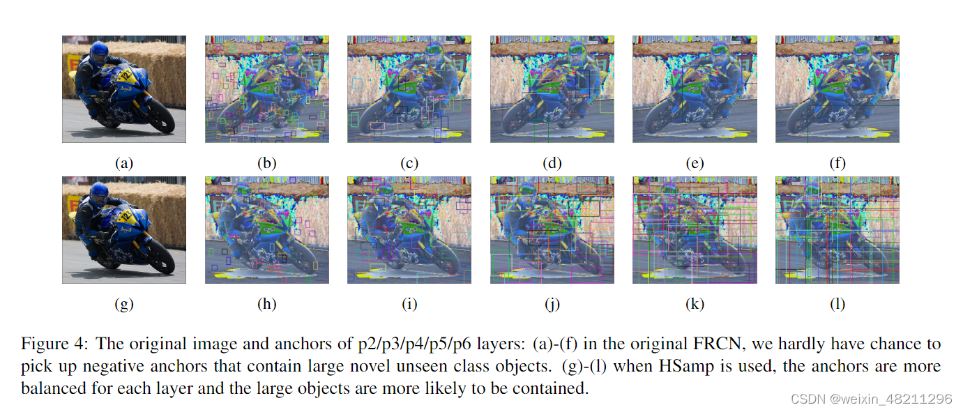
To identify instances of novel unseen classes, we randomly select Ans in a hierarchically balanced way, namely hierarchically sampling (HSamp). That is, if we need to pick up m negative anchors (m<256), we equally assign them to each feature layer so that each layer will have around m/5 anchors. This way, the anchors in each feature layer would share the same possibility for being selected, as shown in Figure. 3b. Therefore, the anchors that belong to the p4 to p6 layers are safely preserved. For example, in Figure. 3b, there are [[120,000], [30,000], [7,500], [1,875], [507]] anchors for p4 to p6 layers in a training batch, and 218 negative anchors are needed. With the original RPN, these 218 An anchors are randomly selected which means the number of An for p6 feature map is only 3. In contrast, when HSamp is used, the number of An is equal for each feature map. We have also visualized the effect of our method in Figure 4. There is hardly any An that contains the motorbike (novel unseen object) when using the original RPN, as shown in Figure. 4a to 4f. However, when HSamp is used, the chance to have an An that contains the motorbike is higher, as shown in Figure. 4g to 4l. We conclude that it is crucial to implement a balanced strategy in sampling negative anchors among all feature layers in order to find potential objects that belong to unseen novel classes. The approach will help us to isolate unseen novel class in-stances as instances that are not similar to the seen classes.
为了识别未见新颖类别的实例，我们以分层平衡的方式随机选择负锚点An，即分层采样（HSamp）。换句话说，如果我们需要挑选出m个负锚点（m<256），我们会将它们均匀分配到每个特征层中，以便每个层大约有m/5个锚点。这样，每个特征层中的锚点都会有相同的可能性被选择，如图3b所示。因此，属于p4到p6层的锚点被安全地保留了。例如，在图3b中，对于一个训练批次，p4到p6层中分别有[[120,000], [30,000], [7,500], [1,875], [507]]个锚点，需要218个负锚点。使用原始RPN时，这218个An锚点是随机选择的，这意味着p6特征图的An数量只有3个。相比之下，当使用HSamp时，每个特征图的An数量是相等的。我们还在图4中可视化了我们方法的效果。如图4a至4f所示，使用原始RPN时，几乎没有任何一个An包含摩托车（未见新颖对象）。然而，当使用HSamp时，含有摩托车的An的机会更高，如图4g至4l所示。我们得出结论，在所有特征层中实施平衡的策略以在其中找到属于未见新颖类别的潜在对象是至关重要的。该方法将帮助我们将未见新颖类别实例与已见类别不相似的实例隔离开来。

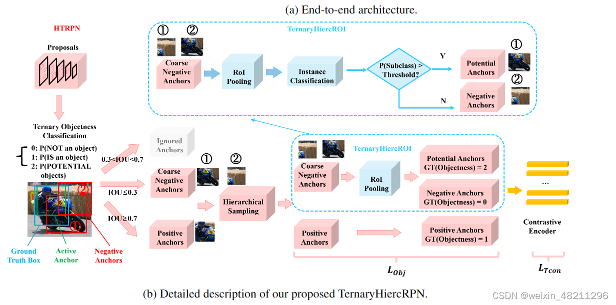
4.2 Hierarchical ternary classification region proposal network (HTRPN)

As mentioned in Section 4.1, faster R-CNN has the ability to recognize a number of potential novel objects that belong to unseen classes, despite the fact that they are unlabelled during training on base class images. We hypothesize that this ability is because of the feature similarity between the features of some novel unseen classes and the base classes. As a result, the model would predict a novel unseen class object as a base class based on its resemblance. In other words, the novel objects contained by the negative anchors could probably have a relatively high classification score towards a base class that resembles them the most. We mark the negative anchors that contain potential novel unseen class objects as potential anchors (Ap), while others are marked as true negative anchors (At n). Our goal is to distinguish between these two subsets.
如第4.1节所述，Faster R-CNN具有识别属于未见类别的一些潜在新颖对象的能力，尽管它们在基础类别图像的训练过程中未被标记。我们假设这种能力是由于一些新颖未见类别的特征与基础类别的特征相似。因此模型会根据它们的相似性将新颖未见类别对象预测为基础类别。换句话说，负锚点中包含的新颖对象可能对与它们最相似的基础类别具有相对较高的分类分数。我们将包含潜在新颖类别对象的负锚点标记为潜在锚点（Ap），而其他的则标记为真负锚点（$A_n^t$）。我们的目标是区分这两个子集。

Figure 5 visualizes our proposed architecture for improving FSOD. To better distinguish the set of Ap from the set of At n during training, instead of performing binary classification to determine objectness in the original RPN, we propose a ternary objectness classification (i.e.,tobj{tobjprei, tobjgt, ioua gt}, where tobjprei are the predicted ternary objectness scores between 0 and 1 for each class i; ground-truth value tobjgt = 0 indicates non-object,tobjgt = 1 represents a true object, tobjgt = 2 represents potential objects from unseen novel classes) so that potential objects that belong to unseen novel classes can be classified as a separate class, as visualized in Figure. 5b. For a training image, after the hierarchical sampling of the coarse negative anchors, we keep these negative anchors for any batch of anchors and perform instance-level sub-classification on them. Here, we set an instance-level classification threshold (T hrecls). If we observe that the classification score is larger than the threshold (P (cls) > T hrecls) for a base class, then we set the anchor as an objectness-positive anchor, and mark its objectness loss with the ground truth of the label 2. For example the motorbike in Figure. 5b, the blue box is the ground truth box, active anchors are in green boxes, while negative anchors are in red boxes. Features of the negative anchors are sent to the RoI pooling layer to see if they could be predicted as a visually similar seen category (e.g. the negative anchor ̈ is predicted as base class “bicycle”, then it is assigned with tobjgt = 2; but for anchor ≠ is kept as tobjgt = 0since it does not pass the T hrecls. We argue that our novel architecture will have a higher FSOD performance.
图5可视化了我们提出的用于改进FSOD的架构。为了在训练过程中更好地区分Ap集合和At n集合，我们提出了一种三元对象性分类（即$\mathrm{tobj}\left\{\text{ tobj }{j}_{\text{pre }}{}^i,\mathrm{tobj}{j}_{gt},io{u}_{gt}^a\right\}$,其中${\text{ tobj }}_{\text{pre }}{}^i$是每个类别i的预测三元对象性分数，在0和1之间；地面实况值$tob{j}_{gt}=0$表示非对象，$tob{j}_{gt}=1$表示真实对象，$tob{j}_{gt}=2$表示来自未见新颖类别的潜在对象），以便属于未见新颖类别的潜在对象可以被分类为一个单独的类别，如图5b所示。对于一个训练图像，在对粗糙负锚点进行分层采样后，我们保留这些负锚点，并对它们进行实例级子分类。在这里，我们设置一个实例级分类阈值（$Thr{e}_{cls}$）。如果我们观察到对于一个基础类别，分类分数大于阈值（P（cls）>$Thr{e}_{cls}$），那么我们将锚点设置为对象性阳性锚点，并将其对象性损失标记为标签2的地面实况。例如，图5b中的摩托车，蓝色框是地面实况框，活跃锚点在绿色框中，而负锚点在红色框中。将负锚点的特征发送到RoI池化层，以查看它们是否可以被预测为视觉上类似的已见类别（例如，负锚点 ̈1被预测为基础类别“自行车”，然后被分配 $tob{j}_{gt}=2$；但对于锚点2 被保留为$tob{j}_{gt}=0$，因为它没有通过$Thr{e}_{cls}$）。我们认为我们的新架构将具有更高的FSOD性能。

In addition, we need customized solutions for the pretraining and fine-tuning when using our proposed HTRPN Considering computational resource limitations, only the top 1000 proposals are used for RoI pooling in traditional RPN. Proposals are ranked by their objectness score oftobjpre1 during the pre-training stage since the model only learns to identify the base classes in this stage. However, in the fine-tuning stage, the tobjpre1 and tobjpre2 are both considered for ranking the proposals, because the objectness of some labeled objects might be predicted as tobjpre2due to knowledge transfer from the pre-training stage. This step is crucial to realize the objectness consistency because the combination of tobjpre1 and tobjpre2 could represent the highly confident proposal and especially improve the possibility of determining positive anchors while inferencing. As shown in Figure 6, if the top two proposals out of the five proposals are ranked only using tobjpre1, then the proposal Ø would be ignored. However, when the top two proposals are ranked by tobjpre1 ⊕ tobjpre2 (operator ⊕could be addition or maximum, here we use maximum, details about ⊕ will be discussed in Appendix), the proposalØ could be correctly included. Such a scheme significantly increases the possibility to dig up the true object as much as possible. As a result, the anchors that contain potential novel unseen class objects are well distinguished from the coarse negative anchors. The ternary RPN will let the model maintain its sensitivity to identify new objects from classes that have never been seen before. In practice, not all potential objects that exist in training datasets are going to be singled out during training and only a subset of them could be found. However, these identified novel unseen class objects still can alleviate the confusion of the model during fewshot learning due to their dissimilarity to the seen classes.
此外，当使用我们提出的HTRPN时，我们需要定制化的解决方案来进行预训练和微调。考虑到计算资源的限制，在传统的RPN中只使用了前1000个提议进行RoI池化。在预训练阶段，提议按照其$tob{j_{pre}}^1$的objectness进行排名，因为模型在这个阶段只学习识别基础类别。然而，在微调阶段，$tob{j_{pre}}^1$和$tob{j_{pre}}^2$都被认为是对proposal的排名，由于从预训练阶段的知识转移过来，一些标记对象的对象性可能被预测为$tob{j_{pre}}^2$。这一步骤对于实现对象性的一致性至关重要，因为$tob{j_{pre}}^1$和$tob{j_{pre}}^2$的组合可以代表高度自信的proposal，并在推理时可以提高确定正锚点的可能性。如图6所示，如果五个提议中的前两个提议仅使用$tob{j_{pre}}^1$进行排名，那么提议4将被忽略。然而，当前两个提议通过$tob{j_{pre}}^1$⊕ $tob{j_{pre}}^2$（⊕运算符可以是加法或最大值，这里我们使用最大值， ⊕的详细信息将在附录中讨论）进行排名时，提议4可以被正确地包括。这样的方案大大增加了挖掘真实对象的可能性。因此，包含潜在新颖未见类别对象的锚点与粗糙负锚点有很好的区分。三元RPN将使模型保持对从未见过的类别中识别新对象的敏感性。在实践中，并不是所有存在于训练数据集中的潜在对象都会在训练过程中被挑选出来，只有其中的一个子集才能被找到。然而，这些被识别出的新颖未见类别对象仍然可以减轻模型在少样本学习期间的混淆，因为它们与已见类别不同。

4个蓝色框是真值框，5个红色框是proposal。该提案4包含一个未标记的新对象椅子。按 $tob{j_{pre}}^1$ ⊕$tob{j_{pre}}^2$ 排名的前 2 个提案可以成功地包含提案 4。

4.3 Contrastive learning on objectness

To further increase the inter-class distances between Aa,At n, and Ap subsets in HTRPN, we also include an objectness contrastive learning head (ConsObj) in our architecture. Inspired by the existing literature [31, 16], the cropped features of proposals are sent into an encoder with their ground truth objectness logits to perform contrastive learning. The features of proposals are encoded as a default 128-dimension feature vector, and then the cosine similarity scores are measured between every two proposals. In this way, the HTRPN would give a higher objectness score.
为了进一步增加HTRPN中Aa、$A_n^t,$和Ap子集之间的类间距离，我们还在我们的架构中包含了一个对象性对比学习头（ConsObj）。受现有文献的启发[31, 16]，proposal的裁剪特征与它们的真实对象性logits一起被送入编码器进行对比学习。proposal的特征被编码为默认的128维特征向量，然后测量每两个proposal之间的余弦相似度分数。通过这种方式，HTRPN会给出一个更高的objectness分数。

4.4 Training Loss

The global total loss is composed of the classification loss (LCls), the bounding box regression loss (LBbox), our ternary objectness loss (LT obj ), and the RoI feature contrastive loss LContra, as described in Equation. 1. TheLContra is computed using the contrastive head as described in FSCE [31]. We set α = 0.5 to be the fixed weight for balancing the contrastive learning loss.
$$\mathcal{L}={\mathcal{L}}_{Cls}+{\mathcal{L}}_{Bbox}+{\mathcal{L}}_{Tobj}+\alpha {\mathcal{L}}_{Contra}(1)$$
全局总损失由分类损失（${\mathcal{L}}_{Cls}$）、边界框回归损失（${\mathcal{L}}_{Bbox})$）、我们的三元对象性损失（${\mathcal{L}}_{Tobj})$）和RoI特征对比损失${\mathcal{L}}_{Contra})$组成，如方程式1所述。${\mathcal{L}}_{Contra})$是使用FSCE中描述的对比头计算的。我们设置α = 0.5作为平衡对比学习损失的固定权重。

Our proposed ternary objectness loss${\mathcal{L}}_{Tobj}$ in Equation. 2 is a sum of the cross entropy objectness loss( ${\mathcal{L}}_{obj}$) and ternary RPN feature contrastive learning loss (${\mathcal{L}}_{Tcon}$). Similar to α in Equation. 1, λ is a balancing factor that is set to be equal 0.5 in our experiments.
$${\mathcal{L}}_{Tobj}={\mathcal{L}}_{Obj}+\lambda {\mathcal{L}}_{Tcon}(2)$$
我们提出的方程式2中的三元对象性损失${\mathcal{L}}_{Tobj}$ 是交叉熵对象性损失（${\mathcal{L}}_{obj}$）和三元RPN特征对比学习损失（${\mathcal{L}}_{Tcon}$）的总和。与方程式1中的α类似，λ是一个平衡因子，在我们的实验中被设置为0.5。

The ternary RPN contrastive learning loss LT con, is defined as an arithmetic mean of the weighted supervised contrastive learning loss Lzi as the following:
$${\mathcal{L}}_{Tcon}=\frac{1}{N_{Prop}}\sum _{i=1}^{N_{Prop}}w(io{u}_{gt}^p)\cdot {\mathcal{L}}_{z_i},(3)$$
三元RPN对比学习损失${\mathcal{L}}_{Tcon}$被定义为加权监督对比学习损失${\mathcal{L}}_{Zi}$的算术平均值，如下所示：

where NP rop represents the number of RPN proposals. Weights w(ioup gt) are assigned by the function g(∗):
w ( i o u g t p ) = I { i o u g t p ≥ ϕ } ⋅ g ( i o u g t p ) , ( 4 ) w(iou_{gt}^p)=\mathcal{I}\{iou_{gt}^p\geq\phi\}\cdot g(iou_{gt}^p),\quad(4) w(iougtp​)=I{iougtp​≥ϕ}⋅g(iougtp​),(4)
其中${\mathcal{N}}_{prop}$表示 RPN 提议的数量。权重$w(io{u}_{gt}^p)$由函数 g(∗) 分配：

where g(∗) = 1 is a good hard-clip [31] and I{∗} is a cut-off function that is 1 when ioup gt ≥ φ , otherwise is 0.Lzi in the RPN proposal contrastive learning loss is given as
L z i = − 1 N o b j g t i − 1 ∑ j = 1 , j ≠ i N P r o p I { o b j g t i = o b j g t j } ⋅ log ⁡ e z i ~ ⋅ z j ~ / τ ∑ k = 1 N P r o p I k ≠ i ⋅ e z i ~ ⋅ z k ~ / τ , ( 5 ) \mathcal{L}_{z_{i}}=\frac{-1}{N_{obj_{gt}^{i}}-1}\sum_{j=1,j\neq i}^{N_{Prop}}\mathcal{I}\{obj_{gt}^{i}=obj_{gt}^{j}\}\cdot\log\frac{e^{\tilde{z_{i}}\cdot\tilde{z_{j}}/\tau}}{\sum_{k=1}^{N_{Prop}}\mathcal{I}_{k\neq i}\cdot e^{\tilde{z_{i}}\cdot\tilde{z_{k}}/\tau}},(5) Lzi​​=Nobjgti​​−1−1​j=1,j=i∑NProp​​I{objgti​=objgtj​}⋅log∑k=1NProp​​Ik=i​⋅ezi​~​⋅zk​~​/τezi​~​⋅zj​~​/τ​,(5)
其中 g(∗) = 1 是一个好的hard-clip函数 [31]， I { ∗ } \mathcal{I}\{*\} I{∗} 是一个截止函数，当 $io{u}_{gt}^p\ge \varphi$时为 1，否则为 0。 RPN 提议对比学习损失中的 ${\mathcal{L}}_{Zi}$给出为

where zi denotes the contrastive feature, obji gt denotes the ground truth ternary objectness label for the i-th proposal, ̃zi denotes normalized features while measuring the cosine distances, and Nobji gt denotes the number of proposals with the same objectness label as obji gt.
其中，$z_i$表示对比特征，$ob{j}_{gt}^i$表示第i个提议的真实三元对象性标签，${\tilde{z}}_i$表示在测量余弦距离时进行了归一化的特征，而$N_{ob{j}_{gt}^i}$表示具有与$ob{j}_{gt}^i$相同对象性标签的提议数量。

5 Experimental Results

5.1 Expeiremntal Setup

我们使用Faster R-CNN作为我们的目标检测模型，并使用ResNet-101作为骨干网络，以及特征金字塔网络（FPN）。评估方案严格遵循与TFA[35]中描述的相同范式。mAP50评估结果分别在基础类别（bAP50）和新见类别（nAP50）上进行计算。我们在PASCAL VOC和COCO数据集上报告我们的结果。在微调阶段，对比学习头的计算方式与FSCE[31]类似。我们使用了四个GPU进行训练。优化器固定为SGD，权重衰减为1e-4，动量为0.9。我们将批量大小设置为16用于所有实验。T hrecls被固定为0.75。这些超参数没有进行微调。在预训练阶段，用于RoI池化的前1000个提议，按第二个对象性对数（表示为对象）进行排序。而在微调阶段，前1000个提议按第二个和第三个对象性对数（表示为潜在对象）的最大值进行排序。有许多现有的FSOD方法。我们将我们的性能与最近开发的一些SOTA FSOD方法的子集进行比较。

5.4. Ablation Study

Firstly, we discuss the effectiveness of our proposed modules separately, including the Hierarchical sampling of the RPN, the ternary objectness classification, and the contrastive head of the objectness. We implemented the ablation study experiment on PASCAL VOC 5-shot scenario. Each proposed module is added to the original network in an accumulated manner. The results are presented in Table. 3. We observe that all our proposed modules are necessary for optimal performance. By adding the HSamp, we can see that a balanced sampling in RPN is necessary, as it provides comprehensive improvement of bAP and nAPduring the pre-training and the fine-tuning stages. We can also observe the results of adding the ternary objectness module indicate that our method will further improve thenAP and do no significant harm to the bAP . While the contrastive objectness part demonstrated that it is a simple yet effective way to help build a stronger RPN that could further improve the bAP and nAP。
首先，我们讨论我们提出的模块的有效性，包括RPN的分层采样、三元对象性分类和对象性对比头。我们在PASCAL VOC 5-shot场景上进行了消融研究实验。每个提出的模块都以累积方式添加到原始网络中。结果如表3所示。我们观察到，我们所有提出的模块都是达到最佳性能所必需的。通过添加HSamp，我们可以看到，在RPN中进行平衡采样是必要的，因为它在预训练和微调阶段都提供了bAP和nAP的全面改善。我们还可以观察到，添加三元对象性模块的结果表明，我们的方法将进一步改善nAP，并对bAP没有明显的伤害。而对象性对比部分表明，这是一种简单而有效的方法，有助于构建一个更强大的RPN，进一步提高bAP和nAP。

模块消融研究。逐步将每个模块添加到基线网络中的效果分别展示。符号*表示我们的再现结果。我们列出了预训练阶段和微调阶段的基础类别mAP50（bAP），以及微调阶段的新类别mAP50（nAP）

Additionally, we study the influence of different hyperparameter T hrecls settings. We use five T hrecls values from 0.05 to 0.95 for training and record the nAP accordingly, as shown in Table. 4. We observe that for lowerT hrecls, more candidate potential novel proposals can be distinguished. However, we have lower confidence and consequently lower quality. However, when a higher threshold T hrecls is used, the number of candidates for potential novel proposals is smaller, which is insufficient to optimize objectness in our framework. As the result indicates,T hrecls = 0.75 is a reasonable value for filtering the candidate proposals relatively well. For additional quantitative analysis please refer to the supplementary materials.
此外，我们研究了不同超参数$Thr{e}_{cls}$设置的影响。我们使用了从0.05到0.95的五个$Thr{e}_{cls}$值进行训练，并相应地记录nAP，如表4所示。我们观察到，对于较低的$Thr{e}_{cls}$，可以区分更多候选的潜在新提议。然而，我们的置信度较低，因此质量较低。然而，当使用较高的阈值$Thr{e}_{cls}$时，潜在新提议的候选数量较少，这不足以优化我们框架中的对象性。正如结果所示，$Thr{e}_{cls}$ = 0.75是一个合理的值，可以相对较好地过滤候选提议。有关更多的定量分析，请参考补充材料。

A Ranking proposals

As mentioned in our main paper Section 4.2, the top 1,000 proposals that are most likely to contain objects are selected for the training according to their objectness logit scores. Since our proposed hierarchical ternary region proposal network (HTRPN) has three objectness scores (tobjpre0 indicates the predicted score of non-object,tobjpre1 represents the score of the true object, tobjpre2represents the score of potential objects from unseen novel classes), we rank the proposals by combing their tobjpre1and tobjpre2, mark as tobjpre1 ⊕ tobjpre2. Operator ⊕could be either arithmetical addition (tobjpre1 + tobjpre2) or maximum (max(tobjpre1, tobjpre2)).
正如我们在主要论文的第4.2节中提到的那样，根据它们的对象性logit分数，选择最有可能包含对象的前1000个提议进行训练。由于我们提出的分层三元区域建议网络（HTRPN）有三个对象性得分 （$tob{j}_{pre}^0$表示非对象的预测得分，$tob{j}_{pre}^1$表示真实对象的得分，$tob{j}_{pre}^2$表示来自未知新类的潜在对象的得分），我们通过组合它们的$tob{j}_{pre}^1$和$tob{j}_{pre}^2$来对提议进行排名，并标记为$tob{j}_{pre}^1$ ⊕ $tob{j}_{pre}^2$。运算符⊕可以是算术加法（$tob{j}_{pre}^1$ + $tob{j}_{pre}^2$）或最大值（max（$tob{j}_{pre}^1$ , $tob{j}_{pre}^2$））

Our examples in Figure. 7 demonstrate the difference between these two types of the operator ⊕. In the image, labeled base class objects (tables and chairs) are in blue boxes. For five exemplary proposals ̈ to ∞ in red boxes with their ternary objectness logit scores, we intend to pick the top 2 of them. If we rank the proposals only by tobjpre1, then the proposals that contain unlabeled potential objects (e.g. proposal 4) will more likely be ignored since they are trained to have higher tobjpre2 score instead of tobjpre1. Therefore, it is necessary to take the tobjpre2 score into account, and according to our HTRPN, the objectness of an object should be presented by tobjpre1 and tobjpre2 together so that the rank of the potential proposal such as Øcould be significantly promoted. However, by the method of tobjpre1 + tobjpre2, the rank of some proposals will be negatively influenced by the negative logit values, such as the proposal ∞. On the contrary, by applying the maximum between tobjpre1 and tobjpre2, the rank of proposal ∞ will not be degraded by the singular negative values.
我们在图7中的示例展示了这两种类型的运算符 ⊕ 之间的区别。在图像中，带有标签的基类对象（桌子和椅子）用蓝色框表示。对于五个示例提议1到 5，用红色框表示它们的三元对象性对数分数，我们打算选择其中排名前2的提议。如果我们仅根据$tob{j}_{pre}^1$ 对提议进行排名，那么包含未标记的潜在对象（例如提议 4）的提议更有可能被忽略，因为它们被训练为具有较高的 $tob{j}_{pre}^2$ 分数而不是 $tob{j}_{pre}^1$。因此，有必要考虑 $tob{j}_{pre}^2$分数，并根据我们的 HTRPN，对象的对象性应该由 $tob{j}_{pre}^1$ 和 $tob{j}_{pre}^2$ 共同表示，以便像4 这样的潜在提议的排名可以显著提升。然而，通过$tob{j}_{pre}^1$ +$tob{j}_{pre}^2$的方法，一些提议的排名将受到负对数值的负面影响，例如提议 5。相反，通过应用$tob{j}_{pre}^1$和 $tob{j}_{pre}^2$ 之间的最大值，提议 5 的排名不会被单一的负值降低。

B. Magnitude of potential novel objects

We record the number of potential objects during the pretraining and fine-tuning stages to demonstrate the statistical concept of the potential objects. Our experiments are implemented on the PASCAL VOC dataset with the 5-shot setting. The instance-level ternary classification threshold is fixed as T hrecls = 0.75. The relation between the number of anchors and the training iteration in the pre-training stage is shown in Figure. 8a, the overall training anchors for each image is 256, as we claimed in 4.1, thus, for a batch size of 16 on 4 GPUs, the overall training anchors on a single GPU would be around (16/4) ∗ 256 = 1024. The negative anchors (blue bars) are the majority, and the number of active anchors (orange bars) is around 0 to 50 for each iteration, which is about 4% of all anchors. However, the number of potential anchors (gray bars) converges with training iterations and stays at around 0 to 5 for each iteration, which indicates our model is getting more stable for recognizing the potential novel objects. Furthermore, as shown in Figure. 8b, during 5-shot fine-tuning, the trend of the potential anchors is as same as in the pre-training stage. However, when transferring to novel classes, the pretrained model tends to predict some labeled novel objects as potential novel objects and the beginning of the fine-tuning stage, which could be considered as the inertia of the pretrained model, therefore, the number of potential anchors is relatively high in the first several iterations of training. This also supports our theory that all true/potential positive ternary objectness of anchors should be presented by the combination of tobjpre1 and tobjpre2. And then the number of potential anchors is gradually stabilized to around 0 to 15 for each iteration, which is about 1.5% of all anchors in an iteration.
我们记录了在预训练和微调阶段潜在对象的数量，以展示潜在对象的统计概念。我们的实验在PASCAL VOC数据集上进行，采用了5-shot设置。实例级别的三元分类阈值被固定为$Thr{e}_{cls}$= 0.75。在预训练阶段，锚点数量与训练迭代之间的关系如图8a所示，每个图像的总训练锚点数为256，正如我们在4.1中所述，因此，对于一个在4个GPU上的批量大小为16的训练，单个GPU上的总训练锚点约为(16/4) * 256 = 1024。负锚点（蓝色柱）占据了大部分，而活动锚点（橙色柱）在每个迭代中大约为0到50个，占所有锚点的约4％。然而，潜在锚点（灰色柱）的数量随着训练迭代的进行而收敛，并在每个迭代中保持在0到5左右，这表明我们的模型在识别潜在新对象方面变得更加稳定。

此外，如图8b所示，在5-shot微调期间，潜在锚点的趋势与预训练阶段相同。然而，在转移到新类别时，预训练模型倾向于在微调阶段的开始将一些带标签的新类别对象预测为潜在的新类别对象，这可以视为预训练模型的惯性，因此，在训练的前几个迭代中，潜在锚点的数量相对较高。这也支持了我们的理论，即所有锚点的真实/潜在正三元对象性应通过$tob{j}_{pre}^1$和$tob{j}_{pre}^2$的组合来呈现。随着训练的进行，潜在锚点的数量逐渐稳定在每个迭代中约0到15个左右，这约占每个迭代中所有锚点的1.5％。

C. Implemented details

当我们对 RPN 和 RoI 池化应用对比学习时，预训练和微调样本的特征空间完全不同，这些对比学习模块的权重不能从预训练模型转移到微调任务。因此，我们从预训练模型中删除权重进行微调训练。Resnet 主干和 RoI 池化的权重在微调期间没有冻结。