人工智能神经网络（Artificial intelligence neural network）之感知器算法

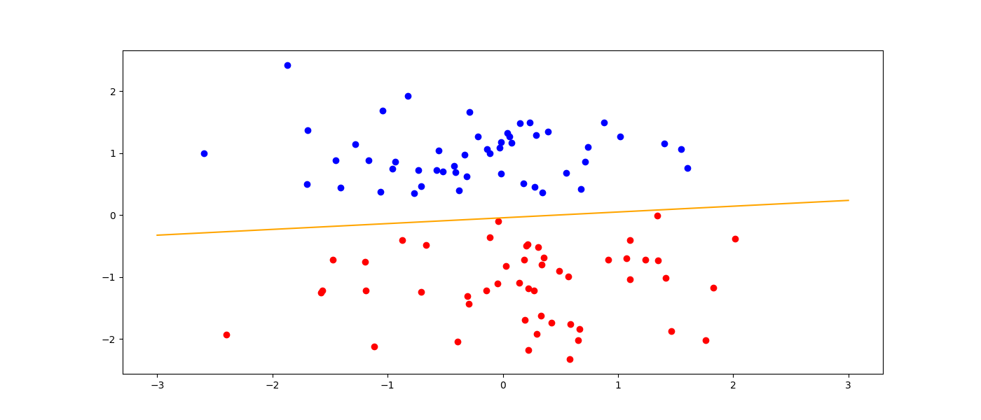
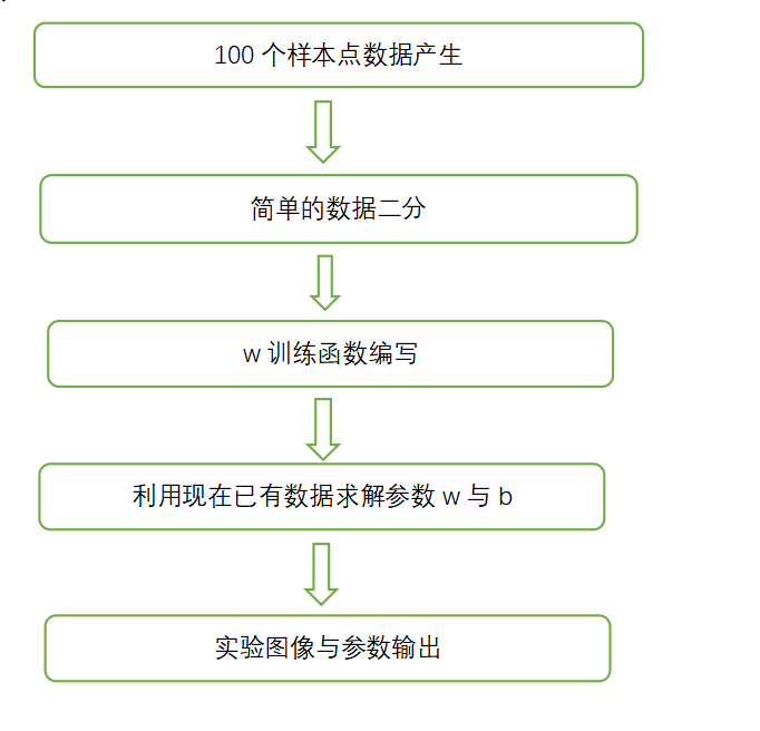
通俗来讲，感知器算法可以完成如下这类线性可分的二分类分类任务。即找出一条超平面，将两类数据进行划分。在输入特征为二维的数据集中，即一条直线。现在自动生成一组数据，并且简单二分，运用算法判断是否线性可分，并且实现感知器算法寻找此条直线，并求解直线相关参数。

感知器算法是一种用于二进制分类的监督学习算法，可以预测数字向量所表示的输入是否属于特定的类。在机器学习的术语中，分类被认为是监督学习的实例，即，其中可观测得到正确识别的训练集，可将之用于训练学习。相应的无监督过程被称为聚类或聚类分析，并且涉及基于固有相似性（例如，被视为多维向量空间中的向量的实例之间的距离）的某种度量将数据分组到类别中。在人工神经网络领域中，感知机也被指为单层的人工神经网络，以区别于较复杂的多层感知机（Multilayer Perceptron）。作为一种线性分类器，（单层）感知机可说是最简单的前向人工神经网络形式。尽管结构简单，感知机能够学习并解决相当复杂的问题。感知机主要的本质缺陷是它不能处理线性不可分问题。我用sklearn.datasets.make_classification 生成了大小为 100的数据集，并在其中按照 8 : 2 的比例随机拆分为了训练集和验证集。在训练过程中，发现可能是因为由 make_classification 生成的数据集太理想，在学习率固定为 0.01 ，通过随机梯度下降进行 1个 epoch 的训练，即可得到非常好的效果，事实上，在 epoch为1，l_rate 为 0.01 时得到准确率为 90% 已经是我多次测试得到最好的结果。

实验结果：

w = [0.81072587, 1.85426] b= 0.04000000000000001

运行步骤：

运行环境:pycharm

运行代码：

'''
JOEY 感知器
'''
import pandas as pd
import numpy as np
import matplotlib.pyplot as plt

from sklearn.datasets import make_classification
from sklearn.model_selection import train_test_split
#100个样本点
x, y = make_classification(n_samples=100, n_features=2, n_redundant=0, n_informative=1, n_clusters_per_class=1)
X_train,X_test,y_train,y_test = train_test_split(x,y,test_size = 0.2,random_state = 2)
# numpy to pandas
X_train = pd.DataFrame(X_train)
X_test = pd.DataFrame(X_test)
y_train = pd.DataFrame(y_train)
y_test = pd.DataFrame(y_test)
y_train[y_train[0] == 0] = -1
y_test[y_test[0] == 0] = -1
# n_samples:生成样本的数量

# n_features=2:生成样本的特征数，特征数=n_informative（） + n_redundant + n_repeated,2类

# n_informative：多信息特征的个数

# n_redundant：冗余信息，informative特征的随机线性组合

# n_clusters_per_class ：某一个类别是由几个cluster构成的
# 绘图显示

#感知器实现算法
class f(object):
    def __init__(self, w_dim, b0=0, l_rate=0.01, epoch=200):
        self.w = np.ones(w_dim, dtype=np.float32)  # w_dim = len(X_train.columns)
        self.b = b0
        self.l_rate = l_rate  # 先固定学习率
        self.epoch = epoch
        self.accuracy = []

    def sign(self, x, w, b) -> int:  # 定义符号函数
        y = np.dot(x, w) + b
        y = float(y)
        if y >= 0:
            return 1
        else:
            return -1

    def Weighted_sum(self, x, w, b) -> float:
        y = np.dot(x, w) + b
        return y

    def fit(self, x_train, y_train):
        #
        self.accuracy.clear()
        accuracy_temp = 0
        for iter_ in range(self.epoch):
            for i in range(len(x_train)):
                xi = x_train.iloc[i]
                yi = y_train.iloc[i]
                accuracy_temp += float(yi) * float(self.Weighted_sum(xi, self.w, self.b))
                # SGD
                # if  self.sign(xi, self.w,self.b) < 0: // 我发现没有这个条件训练的更快，甚至效果更好
                self.w += np.dot(xi, float(yi)) * self.l_rate
                self.b += yi * self.l_rate
            self.accuracy.append(float(accuracy_temp))
            if iter_ %10 == 0:
                print("实验结果:")
                print('w = ',list(self.w),'b=',float(self.b))
            accuracy_temp = 0
    def predict(self,x_test):
        y = []
        for i in range(len(x_test)):
            xi = x_test.iloc[i]
            y.append(self.sign(xi, self.w,self.b))
        return y.copy()

    def score(self,y,label):
        accuracy = 0
        for i in range(len(y)):
            if  y[i] == label.iloc[i][0]:
                accuracy += 1
        return accuracy / len(label)

    pass
#主函数
if __name__ == '__main__':
    perceptron = f(len(X_train.columns),epoch= 10,l_rate= 0.01)
    perceptron.fit(X_train, y_train)
    y_predict = perceptron.predict(X_test)
    # 可视化
    #绘图显示
    mistake_f1_pre = [X_test.iloc[i][0] for i in range(len(X_test)) if y_predict[i] != y_test.iloc[i][0]]
    mistake_f2_pre = [X_test.iloc[i][1] for i in range(len(X_test)) if y_predict[i] != y_test.iloc[i][0]]
    fig = plt.figure(num=1,figsize=(14,6))
    ax1 = fig.add_subplot(111)

    ax1.scatter(x[y==0, 0], x[y==0, 1],c = 'red')
    ax1.scatter(x[y==1, 0], x[y==1, 1],c = 'blue')

    line_x = np.linspace(-3,3,100)  # 这里的范围，方便显示可以自己调

    line_w = -1*(perceptron.w[0]/perceptron.w[1])
    line_b = -1*(float(perceptron.b)/perceptron.w[1])

    line_y = list(map(lambda x : x*line_w + line_b ,line_x))

    ax1.plot(line_x,line_y,c = 'orange')
    print(line_w,line_b)
    plt.show();
    print("实验数据:")
    print(x)