使用 PyTorch 构建 AlexNet

AlexNet 由 Alex Krizhevsky、Ilya Sutskever 和 Geoffrey Hinton 提出，源于他们在 2012 年发表的论文 “ImageNet Classification with Deep Convolutional Neural Networks”。该网络在 2012 年 ImageNet 大规模视觉识别挑战赛 (ILSVRC) 中以显著优势获得冠军。

结构分析

AlexNet 网络中包含 5 个卷积层和 3 个全连接层。

上图中网络结构分为上下两层是因为当年 GTX 580 仅有 3GB 显存，所以需要采用两张 GPU 分两路运算。而现在单块 GPU 的显存和算力都完全足够，因此完全可以在一块显卡上进行训练和推理。

在 AlexNet 的原始论文中提到图像的输入尺寸是 224x224，但 AlexNet 的 Caffe 代码实现中，输入尺寸是 227x227。这是由于在第一个卷积层中使用了步长为 4 的卷积核，如果输入尺寸是 224x224，则输出尺寸无法被整除。为了避免这种情况，代码实现将输入尺寸调整为 227x227。也有一种说法是，输入尺寸是 224x224，然后 padding 为 1 和 2，也就是在上方和左侧添加一行/列零，下方和右侧添加两行/列零，这样输出尺寸也为 (96, 55, 55)，其中 55=224−11+1+24+1。后续输入尺寸使用 227x227。

层数	类型	Kernel Numbers	尺寸 (C, H, W)	Padding	Stride	输出尺寸	计算
	RGB 图像		(3, 227, 227)
1	卷积层	48×2=96	(3, 11, 11)	0	4	(96, 55, 55)	55=227−11+2×04+1
2	最大池化层		(96, 3, 3)	0	2	(96, 27, 27)	27=55−3+2×02+1
3	卷积层	128×2=256	(96, 5, 5)	2	1	(256, 27, 27)	27=27−5+2×21+1
4	最大池化层		(256, 3, 3)	0	2	(256, 13, 13)	13=27−3+2×02+1
5	卷积层	192×2=384	(256, 3, 3)	1	1	(384, 13, 13)	13=13−3+2×11+1
6	卷积层	192×2=384	(384, 3, 3)	1	1	(384, 13, 13)	13=13−3+2×11+1
7	卷积层	128×2=256	(384, 3, 3)	1	1	(256, 13, 13)	13=13−3+2×11+1
8	最大池化层		(256, 3, 3)	0	2	(256, 6, 6)	6=13−3+2×02+1
9	全连接层					4096
10	全连接层					4096
11	全连接层					1000

创新

AlexNet 的主要创新点包括以下几个方面：

1. 使用 ReLU 激活函数：AlexNet 首次在深度卷积神经网络中成功应用 ReLU 作为激活函数，取代了传统的 Sigmoid 函数。这一改变显著提高了训练速度，并解决了深层网络中的梯度消失问题。
2. Dropout 技术：在全连接层中引入 Dropout，通过随机忽略一部分神经元来减少过拟合。
3. 重叠的最大池化：AlexNet 在池化层中使用最大池化而非平均池化，并且采用了重叠的池化策略，以增强特征的表示能力。这种方法提高了模型的泛化能力。以往池化的大小 PoolingSize 与步长 stride 一般是相等的，例如：图像大小为 256x256，PoolingSize=2×2，stride=2，这样可以使图像或是 FeatureMap 大小缩小一倍变为 128，此时池化过程没有发生层叠。但是 AlexNet 采用了层叠池化操作，即 PoolingSize > stride。这种操作非常像卷积操作，可以使相邻像素间产生信息交互和保留必要的联系。
4. 局部响应归一化（LRN）：通过增强高响应神经元的活动并抑制低响应神经元，进一步提高了模型的表现力和泛化能力。后来证明该步骤起到的作用很小，所以就很少使用。
5. GPU 并行计算：AlexNet 利用 GPU 的并行计算能力，显著加速了训练过程。
6. 网络层数增加：在随后的神经网络发展过程中，AlexNet 逐渐让研究人员认识到网络深度对性能的巨大影响。当然，这种思考的重要节点出现在 VGG 网络，但是很显然从 AlexNet 为起点就已经开始了这项工作。

步骤

在编写代码之前，我们先来梳理一下流程步骤：

1. 下载 Imagenette 数据集，将其分为训练集、验证集和测试集。
2. 搭建 AlexNet 模型。
3. 使用训练集训练模型，计算损失，并在每次迭代后使用验证集评估模型性能。
4. 根据验证集性能选择最佳模型并导出。
5. 导入模型权重，在测试集上进行测试，并计算准确率。

环境

我在 Colab 下编写代码，使用 T4 GPU 和 PyTorch，以下是一些准备：

1 2 3 4 5

import torch import torchvision import torch.nn as nn import torch.optim as optim from torch.utils.data import DataLoader, random_split

1 2 3 4 5 6 7 8 9 10 11 12

torch.__version__ # '2.4.0+cu121' device = "cuda" if torch.cuda.is_available() else "cpu" device # 'cuda' seed = 42 if device == "cpu": torch.manual_seed(seed) if device == "cuda": torch.cuda.manual_seed(seed)

数据集

原论文中使用了 ImageNet 数据集，但该数据集还是太大了，很难有足够的算力和时间去训练模型。因此我选择了 Imagenette 数据集，它是 ImageNet 的子集，该数据集中包含了 10 个容易区分的类别，训练集包含 9469 张图片，验证集包含 3925 张图片。Imagenette 没有提供测试集。以下是预处理和下载数据集的代码：

1 2 3 4 5 6 7 8 9 10 11 12 13 14 15 16 17

train_transform = transforms.Compose([ transforms.Resize(256), transforms.RandomCrop(227), transforms.RandomHorizontalFlip(), transforms.ToTensor(), transforms.Normalize(mean=[0.485, 0.456, 0.406], std=[0.229, 0.224, 0.225]) ]) val_transform = transforms.Compose([ transforms.Resize(256), transforms.CenterCrop(227), transforms.ToTensor(), transforms.Normalize(mean=[0.485, 0.456, 0.406], std=[0.229, 0.224, 0.225]) ]) train_set = datasets.Imagenette(root="./dataset", split="train", download=True, transform=train_transform) val_set = datasets.Imagenette(root="./dataset", split="val", download=False, transform=val_transform)

我们从验证集中拿出一半作为测试集：

1 2 3

test_size = int(0.5 * len(val_set)) new_val_size = len(val_set) - test_size val_set, test_set = random_split(val_set, [new_val_size, test_size])

查看用例

使用 Matplotlib 来查看一个训练用例图像。

1 2 3 4 5

import matplotlib.pyplot as plt plt.imshow(train_set[0][0].permute(1, 2, 0).numpy()) plt.title(f"Label: {train_set.classes[train_set[0][1]][0]}") plt.show()

数据加载

1 2 3

train_loader = DataLoader(dataset=train_set, batch_size=128, shuffle=True) val_loader = DataLoader(dataset=val_set, batch_size=128, shuffle=False) test_loader = DataLoader(dataset=test_set, batch_size=128, shuffle=False)

模型构建 www.cqzlsb.com

先构建一个原版 AlexNet 模型。

1 2 3 4 5 6 7 8 9 10 11 12 13 14 15 16 17 18 19 20 21 22 23 24 25 26 27 28 29 30 31 32 33

class AlexNet(nn.Module): def __init__(self, num_classes: int = 1000, dropout: float = 0.5) -> None: super().__init__() self.features = nn.Sequential( nn.Conv2d(3, 96, kernel_size=11, stride=4, padding=0), nn.ReLU(inplace=True), nn.MaxPool2d(kernel_size=3, stride=2), nn.Conv2d(96, 256, kernel_size=5, stride=1, padding=2), nn.ReLU(inplace=True), nn.MaxPool2d(kernel_size=3, stride=2), nn.Conv2d(256, 384, kernel_size=3, stride=1, padding=1), nn.ReLU(inplace=True), nn.Conv2d(384, 384, kernel_size=3, stride=1, padding=1), nn.ReLU(inplace=True), nn.Conv2d(384, 256, kernel_size=3, stride=1, padding=1), nn.ReLU(inplace=True), nn.MaxPool2d(kernel_size=3, stride=2), ) self.classifier = nn.Sequential( nn.Dropout(p=dropout), nn.Linear(256 * 6 * 6, 4096), nn.ReLU(inplace=True), nn.Dropout(p=dropout), nn.Linear(4096, 4096), nn.ReLU(inplace=True), nn.Linear(4096, num_classes), ) def forward(self, x: torch.Tensor) -> torch.Tensor: x = self.features(x) x = torch.flatten(x, 1) x = self.classifier(x) return x

使用 print(AlexNet()) 来打印一下模型：

1 2 3 4 5 6 7 8 9 10 11 12 13 14 15 16 17 18 19 20 21 22 23 24 25 26

AlexNet( (features): Sequential( (0): Conv2d(3, 96, kernel_size=(11, 11), stride=(4, 4)) (1): ReLU(inplace=True) (2): MaxPool2d(kernel_size=3, stride=2, padding=0, dilation=1, ceil_mode=False) (3): Conv2d(96, 256, kernel_size=(5, 5), stride=(1, 1), padding=(2, 2)) (4): ReLU(inplace=True) (5): MaxPool2d(kernel_size=3, stride=2, padding=0, dilation=1, ceil_mode=False) (6): Conv2d(256, 384, kernel_size=(3, 3), stride=(1, 1), padding=(1, 1)) (7): ReLU(inplace=True) (8): Conv2d(384, 384, kernel_size=(3, 3), stride=(1, 1), padding=(1, 1)) (9): ReLU(inplace=True) (10): Conv2d(384, 256, kernel_size=(3, 3), stride=(1, 1), padding=(1, 1)) (11): ReLU(inplace=True) (12): MaxPool2d(kernel_size=3, stride=2, padding=0, dilation=1, ceil_mode=False) ) (classifier): Sequential( (0): Dropout(p=0.5, inplace=False) (1): Linear(in_features=9216, out_features=4096, bias=True) (2): ReLU(inplace=True) (3): Dropout(p=0.5, inplace=False) (4): Linear(in_features=4096, out_features=4096, bias=True) (5): ReLU(inplace=True) (6): Linear(in_features=4096, out_features=1000, bias=True) ) )

权重初始化

We initialized the weights in each layer from a zero-mean Gaussian distribution with standard deviation 0.01. We initialized the neuron biases in the second, fourth, and fifth convolutional layers, as well as in the fully-connected hidden layers, with the constant 1. This initialization accelerates the early stages of learning by providing the ReLUs with positive inputs. We initialized the neuron biases in the remaining layers with the constant 0.

根据原论文中关于权重初始化的描述，我们理论上应该在模型构建时实现以下权重初始化的代码：

1 2 3 4 5 6 7 8 9 10 11 12 13 14 15 16 17 18 19 20 21 22 23 24 25 26 27 28 29 30 31 32

class AlexNet(nn.Module): def __init__(self, num_classes: int = 1000, dropout: float = 0.5, init_weights=True) -> None: super().__init__() self.features = nn.Sequential( # ... ) self.classifier = nn.Sequential( # ... ) if init_weights: self._initialize_weights() def forward(self, x: torch.Tensor) -> torch.Tensor: # ... def _initialize_weights(self): for m in self.modules(): if isinstance(m, nn.Conv2d): nn.init.normal_(m.weight, mean=0, std=0.01) if m.bias is not None: nn.init.constant_(m.bias, 0) elif isinstance(m, nn.Linear): nn.init.normal_(m.weight, mean=0, std=0.01) nn.init.constant_(m.bias, 0) conv_layers = [module for module in self.features if isinstance(module, nn.Conv2d)] for i in [1, 3, 4]: nn.init.constant_(conv_layers[i].bias, 1) for i in range(len(self.classifier) - 1): if isinstance(self.classifier[i], nn.Linear): nn.init.constant_(self.classifier[i].bias, 1)

然而在实际运行时我发现以上方式会让模型没法快速收敛，所以这里就不按照原论文进行权重初始化。

超参数设置

关于超参数设置在原论文中的第 5 节 “Details of learning”：

We trained our models using stochastic gradient descent with a batch size of 128 examples, momentum of 0.9, and weight decay of 0.0005.

We used an equal learning rate for all layers, which we adjusted manually throughout training. The heuristic which we followed was to divide the learning rate by 10 when the validation error rate stopped improving with the current learning rate. The learning rate was initialized at 0.01 and reduced three times prior to termination.

根据以上描述，weight decay 为 0.0005，momentum 为 0.9，batch size 为 128，这里我把学习率固定为 0.01 不再变化。

训练和验证

损失函数使用 CrossEntropy，优化器使用 SGD 与原论文一致。

1 2 3 4 5 6 7 8 9 10 11 12 13 14 15 16 17 18 19 20 21 22 23 24 25 26 27 28 29 30 31 32 33 34 35 36 37 38 39 40 41 42 43 44 45 46 47 48 49 50 51 52 53 54 55 56 57

model = AlexNet(num_classes=10).to(device) loss_fn = nn.CrossEntropyLoss() optimizer = optim.SGD(model.parameters(), lr=0.01, weight_decay=0.0005, momentum=0.9) epochs = 60 best_val_accuracy = 0.0 best_val_loss = 1.0 patience = 5 epochs_without_improvement = 0 for epoch in range(epochs): model.train() train_loss = 0.0 for batch_idx, (data, target) in enumerate(train_loader): data, target = data.to(device), target.to(device) optimizer.zero_grad() output = model(data) loss = loss_fn(output, target) loss.backward() optimizer.step() train_loss += loss.item() train_loss /= len(train_set) model.eval() val_loss = 0.0 val_correct = 0 with torch.inference_mode(): for data, target in val_loader: data, target = data.to(device), target.to(device) output = model(data) val_loss += loss_fn(output, target).item() pred = output.argmax(dim=1, keepdim=True) val_correct += pred.eq(target.view_as(pred)).sum().item() val_loss /= len(val_set) val_accuracy = 100.0 * val_correct / len(val_set) print(f"Epoch {epoch+1}/{epochs}, Train Loss: {train_loss:.4f}, Val Loss: {val_loss:.4f}, Val Accuracy: {val_accuracy:.2f}%") if val_accuracy > best_val_accuracy and val_loss < best_val_loss: best_val_accuracy = val_accuracy best_val_loss = val_loss torch.save(model.state_dict(), "alexnet.pth") epochs_without_improvement = 0 else: epochs_without_improvement += 1 if epochs_without_improvement >= patience: print(f"Early stopping at epoch {epoch+1}!") break

运行结果如下：

1 2 3 4 5 6 7 8 9 10 11 12 13 14 15 16 17 18 19 20 21 22 23 24 25 26 27 28 29 30

Epoch 1/60, Train Loss: 0.0180, Val Loss: 0.0187, Val Accuracy: 10.14% Epoch 2/60, Train Loss: 0.0174, Val Loss: 0.0173, Val Accuracy: 20.58% Epoch 3/60, Train Loss: 0.0159, Val Loss: 0.0156, Val Accuracy: 32.71% Epoch 4/60, Train Loss: 0.0149, Val Loss: 0.0143, Val Accuracy: 38.51% Epoch 5/60, Train Loss: 0.0138, Val Loss: 0.0137, Val Accuracy: 43.30% Epoch 6/60, Train Loss: 0.0126, Val Loss: 0.0117, Val Accuracy: 50.38% Epoch 7/60, Train Loss: 0.0114, Val Loss: 0.0106, Val Accuracy: 56.90% Epoch 8/60, Train Loss: 0.0102, Val Loss: 0.0100, Val Accuracy: 59.14% Epoch 9/60, Train Loss: 0.0096, Val Loss: 0.0093, Val Accuracy: 62.35% Epoch 10/60, Train Loss: 0.0089, Val Loss: 0.0087, Val Accuracy: 65.77% Epoch 11/60, Train Loss: 0.0087, Val Loss: 0.0083, Val Accuracy: 66.58% Epoch 12/60, Train Loss: 0.0081, Val Loss: 0.0094, Val Accuracy: 62.25% Epoch 13/60, Train Loss: 0.0077, Val Loss: 0.0075, Val Accuracy: 71.22% Epoch 14/60, Train Loss: 0.0073, Val Loss: 0.0074, Val Accuracy: 70.15% Epoch 15/60, Train Loss: 0.0069, Val Loss: 0.0069, Val Accuracy: 72.69% Epoch 16/60, Train Loss: 0.0068, Val Loss: 0.0068, Val Accuracy: 72.90% Epoch 17/60, Train Loss: 0.0063, Val Loss: 0.0077, Val Accuracy: 70.66% Epoch 18/60, Train Loss: 0.0065, Val Loss: 0.0066, Val Accuracy: 73.36% Epoch 19/60, Train Loss: 0.0059, Val Loss: 0.0065, Val Accuracy: 74.68% Epoch 20/60, Train Loss: 0.0056, Val Loss: 0.0060, Val Accuracy: 76.52% Epoch 21/60, Train Loss: 0.0058, Val Loss: 0.0065, Val Accuracy: 74.07% Epoch 22/60, Train Loss: 0.0052, Val Loss: 0.0067, Val Accuracy: 74.89% Epoch 23/60, Train Loss: 0.0051, Val Loss: 0.0056, Val Accuracy: 78.55% Epoch 24/60, Train Loss: 0.0049, Val Loss: 0.0056, Val Accuracy: 79.16% Epoch 25/60, Train Loss: 0.0048, Val Loss: 0.0060, Val Accuracy: 77.79% Epoch 26/60, Train Loss: 0.0045, Val Loss: 0.0059, Val Accuracy: 77.28% Epoch 27/60, Train Loss: 0.0044, Val Loss: 0.0054, Val Accuracy: 78.86% Epoch 28/60, Train Loss: 0.0044, Val Loss: 0.0055, Val Accuracy: 78.55% Epoch 29/60, Train Loss: 0.0041, Val Loss: 0.0056, Val Accuracy: 79.52% Early stopping at epoch 29!

这里使用了第 24 轮的模型权重。

测试

让我们导入模型权重并测试：

1 2 3 4 5 6 7 8 9 10 11 12 13 14 15 16 17 18 19 20 21 22 23 24 25 26

test_model = AlexNet(num_classes=10).to(device) test_model.load_state_dict(torch.load("alexnet.pth")) test_loss = 0.0 correct = 0 all_predictions = [] all_targets = [] test_model.eval() with torch.inference_mode(): for data, target in test_loader: data, target = data.to(device), target.to(device) output = test_model(data) test_loss += loss_fn(output, target).item() pred = output.argmax(dim=1, keepdim=True) correct += pred.eq(target.view_as(pred)).sum().item() all_predictions.extend(pred.cpu().numpy()) all_targets.extend(target.cpu().numpy()) test_loss /= len(test_set) accuracy = 100.0 * correct / len(test_set) print(f"Test Loss: {test_loss:.4f}, Accuracy: {accuracy:.2f}%") # Test Loss: 0.0057, Accuracy: 77.68%

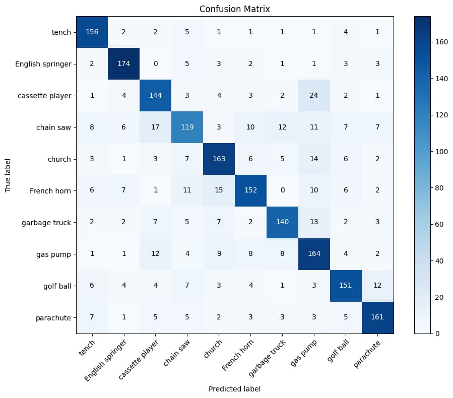
混淆矩阵

最后通过混淆矩阵来可视化模型在测试集上预测的结果：

1 2 3 4 5 6 7 8 9 10 11 12 13 14 15 16 17 18 19 20 21 22 23 24 25 26 27 28 29 30

import numpy as np from sklearn.metrics import confusion_matrix cm = confusion_matrix(all_targets, all_predictions) class_names = ['tench', 'English springer', 'cassette player', 'chain saw', 'church', 'French horn', 'garbage truck', 'gas pump', 'golf ball', 'parachute'] fig, ax = plt.subplots(figsize=(10, 8)) im = ax.imshow(cm, interpolation='nearest', cmap=plt.cm.Blues) ax.figure.colorbar(im, ax=ax) ax.set(xticks=np.arange(cm.shape[1]), yticks=np.arange(cm.shape[0]), xticklabels=class_names, yticklabels=class_names, title='Confusion Matrix', ylabel='True label', xlabel='Predicted label') plt.setp(ax.get_xticklabels(), rotation=45, ha="right", rotation_mode="anchor") thresh = cm.max() / 2. for i in range(cm.shape[0]): for j in range(cm.shape[1]): ax.text(j, i, format(cm[i, j], 'd'), ha="center", va="center", color="white" if cm[i, j] > thresh else "black") fig.tight_layout() plt.show()