吴恩达-python机器学习代码-线性回归笔记

import pandas as pd
import numpy as np
import matplotlib.pyplot as plt

一、单变量线性回归

1、计算代价函数cost function

data=pd.read_csv('/Users/appleguanliyuan/Desktop/yokin_data_analyst_learning_materials/Matalab/machine-learning-ex/ex1/ex1data1.txt',header=None,names=['population','profit'])
data.head()

	population	profit
0	6.1101	17.5920
1	5.5277	9.1302
2	8.5186	13.6620
3	7.0032	11.8540
4	5.8598	6.8233

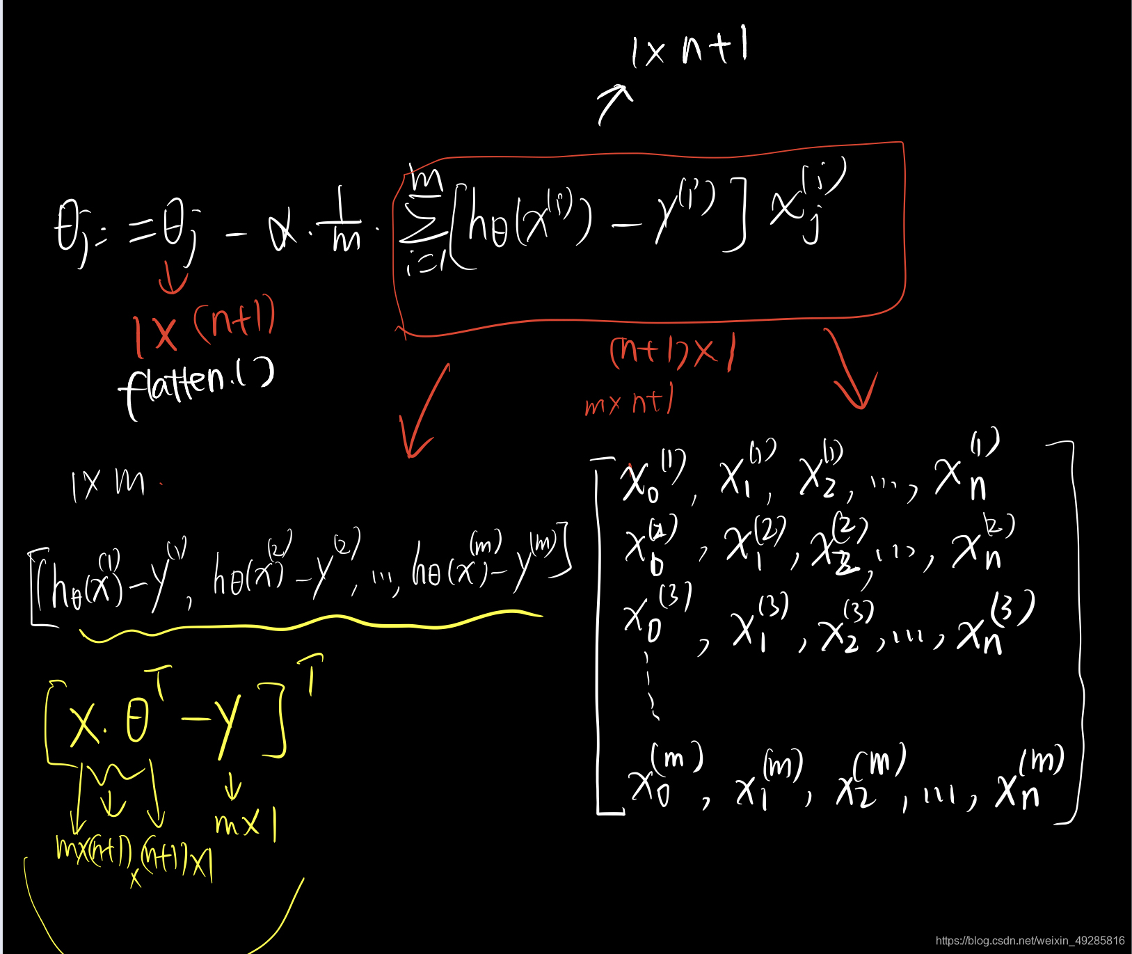
def computeCost(X, y, theta): #注意，这里传入的theta和X,y都应该为matrix形式，以为矩阵想乘直接用*即可，数组则需要.dot()
    inner = np.power(((X * theta.T) -  y), 2)
    return np.sum(inner) / (2 * len(X))

((X * theta.T).T - y)*X 的形式为：

data.insert(0, 'Ones', 1) #插入一列 1
data.head()

	Ones	population	profit
0	1	6.1101	17.5920
1	1	5.5277	9.1302
2	1	8.5186	13.6620
3	1	7.0032	11.8540
4	1	5.8598	6.8233

# set X (training data) and y (target variable)
cols = data.shape[1]  # 列数
X = data.iloc[:,0:cols-1]  # 取前cols-1列，即输入向量
y = data.iloc[:,cols-1:cols] # 取最后一列，即目标向量

#转换为矩阵形式
X = np.matrix(X.values)
y = np.matrix(y.values)
theta = np.matrix([0,0])

X.shape, theta.shape, y.shape
# ((97, 2), (1, 2), (97, 1))

((97, 2), (1, 2), (97, 1))

theta为0时的代价函数

computeCost(X, y, theta) # 32.072733877455676

32.072733877455676

2、梯度下降函数 gradient descent function

def gradientDescent(X,y,theta,alpha,iterations):#需要传入学习几率，梯度下降次数，参数值，X的值和因变量的值
#都要确保传入的是矩阵！    

#暂存theta，为满足后续同时更新需要
    theta_temp=np.matrix(np.zeros(theta.shape)) #初始化赋值为0的theta矩阵

    #参数theta的个数
    theta_num=int(theta.flatten().shape[1])  #flatten函数是把数组或矩阵降为一维，横着降为一维后，shape[1]表示取列数，即个数
     
    cost=np.zeros(iterations) #初始化一个ndarray,包含每次循环的cost
    m=X.shape[0] #样本数量m
    for i in range(iterations):#i从0开始，结束值为iterations-1
        #利用向量化求解
        theta_temp=theta-(alpha/m)*(X*theta.T-y).T*X #注意，为1*n+1的向量
        theta=theta_temp
        cost[i]=computeCost(X,y,theta)
    return theta,cost
    

#已知：
alpha=0.01
iterations=1500
#则：
final_theta,cost=gradientDescent(X,y,theta,alpha,iterations)
final_theta

matrix([[-3.63029144,  1.16636235]])

computeCost(X,y,final_theta)

4.483388256587726

3、可视化代价函数

plt.title("Visualizing J(θ)")
plt.xlabel("iterations")
plt.ylabel("cost")
plt.plot(np.arange(iterations), cost, color="red")
# np.arrange(iterations)为迭代轮数，cost为每轮的损失值，这个计算要插入到梯度下降过程中，计算和记录。

[<matplotlib.lines.Line2D at 0x7fddc8329250>]

​

​

二、多变量线性回归

data2=pd.read_csv('/Users/appleguanliyuan/Desktop/yokin_data_analyst_learning_materials/Matalab/machine-learning-ex/ex1/ex1data2.txt',header=None,names=['Size','Bedrooms','Price'])

data2.head()

	Size	Bedrooms	Price
0	2104	3	399900
1	1600	3	329900
2	2400	3	369000
3	1416	2	232000
4	3000	4	539900

1、特征归一化

data2[['Size','Bedrooms']]=(data2[['Size','Bedrooms']]-data2[['Size','Bedrooms']].mean())/data2[['Size','Bedrooms']].std()
data2.head() #'注意，price因变量不用归一化'

	Size	Bedrooms	Price
0	0.130010	-0.223675	399900
1	-0.504190	-0.223675	329900
2	0.502476	-0.223675	369000
3	-0.735723	-1.537767	232000
4	1.257476	1.090417	539900

2、多元回归

# add ones column
data2.insert(0,'Ones',1)

#set X(training data) and y(target variable)
cols=data2.shape[1]
X2=data2.iloc[:,0:cols-1]
y2=data2.iloc[:,cols-1:cols]

#convert to matrices and initialize theta
X2=np.matrix(X2.values)
y2=np.matrix(y2.values)
theta2=np.matrix([0,0,0])  

#perform linear regression on the data set
theta_of_multiple_regression,cost2=gradientDescent(X2,y2,theta2,alpha,iterations)

#get the cost of the model
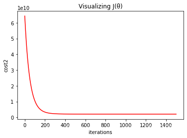
computeCost(X2,y2,theta_of_multiple_regression)
#iterations=1500, alpha=0.01的时候的Cost

2043283576.6373606

plt.title("Visualizing J(θ)")
plt.xlabel("iterations")
plt.ylabel("cost2")
plt.plot(np.arange(iterations), cost2, color="red")
#np.arrange(iterations)为迭代轮数，cost为每轮的损失值，这个计算要插入到梯度下降过程中，计算和记录。

[<matplotlib.lines.Line2D at 0x7fddc8518ac0>]

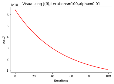
3、改变iterations和alpha的值时

#当iterations=100， alpha=0.01时，
iterations=100
alpha=0.01
theta3,cost3=gradientDescent(X2,y2,theta2,alpha,iterations)
theta3

matrix([[215810.61679138,  61384.03125186,  20273.55045338]])

#改变iterations后，先调用梯度下降函数计算出theta的值，然后带入computeCost'函数
computeCost(X2,y2,theta3) 

10621009943.600248

plt.title("Visualizing J(θ),iterations=100,alpha=0.01")
plt.xlabel("iterations")
plt.ylabel("cost3")
plt.plot(np.arange(iterations), cost3, color="red")
#下图可以看出可以增加alpha的值

[<matplotlib.lines.Line2D at 0x7fddc8579ee0>]

​

三、 正规方程Normal equation求解

def normalEqn(X,y):
    theta=np.linalg.inv(X.T*X)*X.T*y
    return theta
#theta的值此时，算出来时 (n+1)*1维度

final_theta2=normalEqn(X,y)
final_theta3=final_theta2.flatten() #转化为1*n+1,因为computeCost方程会再次转置为(n+1)*1
final_theta3

matrix([[-3.89578088,  1.19303364]])

computeCost(X, y, final_theta3)

4.476971375975179

参考：https://blog.csdn.net/Cowry5/article/details/80174130

修改：对原文正则方程中取消了点乘，增加了不同iterations和alpha的可视化，增加了矩阵相乘的可视化