【强化学习】从蒙特卡洛→SARSA，从Q-Learning→Double Q-Learning

ɛ-greedy-search

强化学习里重要的问题：Exploration vs Exploitation

放弃现有的经验而去探索新路径 还是 坚持现有的最有经验？

def policy(state, Q_table, eps = 0.05):
    """
    If you are using a Q_table to evaluate the (state, action),
    then you need the epsilion to give your agent some chance to explore (or use a sampling Parameter).
    """
	# if random.random() < eps:  # for Q_table is a numpy
    if random.random() < eps or not state in Q_table:  # for Q_table is a dict
        return random.ranint(len(Q_table[state]))
    else:
        return np.argmax(Q_table[state])

ɛ-greedy-search能够让我们比较简单地缓和exploration-exploitation。

Markov Decision Chain

Markov 性质 (Markov Property)

• 在马尔可夫性质下，一个状态被称为"马尔可夫状态"，如果在该状态下，未来的状态（以及未来的奖励）仅依赖于当前状态和采取的动作，而不依赖于先前的状态和动作序列。
  • 简而言之，如果一个系统满足马尔可夫性质，那么当前状态包含了过去的所有信息，以便对未来的状态和奖励进行预测。

存在一种序列问题场景，存在这样的情况

• 情况1：此时此刻的状态 (state_t)，被且仅被上一时刻的state_{t-1}和action_{t-1}，和一个随机变量 (系统存在) 所决定

  memory-less 无记忆过程

  马尔科夫过程 Markov，state( position, v, a ) -> state( position, v, a, key[False/True],… )
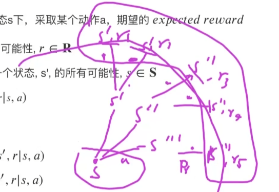
  $$\sum _{a\in A,s^{\prime }\in S,r\in R}Pr(s^{\prime },r|(s,a))=1$$

  考虑一个赌博机（老虎机）游戏的例子。如果游戏的状态只包括当前的老虎机图案和玩家之前的动作（拉杆或不拉杆），并且未来的奖励仅依赖于当前状态和动作（即，老虎机的图案和拉杆的选择），那么这个游戏就满足马尔可夫性质，状态是Markov状态。

• 情况2：此时此刻的状态 (state_t)，被上一时刻的state_{t-1}和action_{t-1}决定，同时也有可能被另外一个/某些states所决定

  memory 有记忆过程

  数学上非常难处理

  比如游戏的状态还包括玩家的所有历史动作和奖励，未来的奖励不仅依赖于当前状态和动作，还依赖于玩家的过去动作和奖励序列，那么这个游戏就不满足马尔可夫性质，状态是非Markov状态。

Math Exercise

第一组

s, a, s'都是已知的，假设r的所有可能为R
$$P{r}_1(s^{\prime }|s,a)\_\_\_\_P{r}_2(s^{\prime },r|s,a)$$
A. ==
B. <=
C. >=
D.不一定

C

可以这么理解两者的关系
$$Pr(s^{\prime }|s,a)=\sum _{r\in R}Pr(s^{\prime },r|s,a)$$

第二组

s'和Pr(s',r|s,a)是已知的，假设r的所有可能为R
$$r(a,s)=\_\_\_\_\_\_\_\_$$
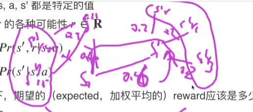
问在某个状态s下，采取某个动作a，期望的 expected reward (即加权平均)

A.
KaTeX parse error: No such environment: flalign at position 8: \begin{̲f̲l̲a̲l̲i̲g̲n̲}̲ &\sum_{r\in R}…
B.
KaTeX parse error: No such environment: flalign at position 8: \begin{̲f̲l̲a̲l̲i̲g̲n̲}̲ &\sum_{s'\in S…
C.
KaTeX parse error: No such environment: flalign at position 8: \begin{̲f̲l̲a̲l̲i̲g̲n̲}̲ &\sum_{r\in R,…
D.
KaTeX parse error: No such environment: flalign at position 8: \begin{̲f̲l̲a̲l̲i̲g̲n̲}̲ &\sum_{r\in R,…

D

第三组

s, a, s',Pr(s',r|s,a)和Pr(s'|s,a)是已知的 (即已知在某个状态s下采取了动作a，达到了s')，假设r的所有可能为R
$$r(a,s,s^{\prime })=\_\_\_\_\_\_\_\_$$
问在 (a,s,s')下，期望的 expected reward (即加权平均)

A.
KaTeX parse error: No such environment: flalign at position 8: \begin{̲f̲l̲a̲l̲i̲g̲n̲}̲ &\sum_{r\in R}…
B.
KaTeX parse error: No such environment: flalign at position 8: \begin{̲f̲l̲a̲l̲i̲g̲n̲}̲ &\sum_{r\in R}…
C.
KaTeX parse error: No such environment: flalign at position 8: \begin{̲f̲l̲a̲l̲i̲g̲n̲}̲ &\sum_{r\in R}…
D.
KaTeX parse error: No such environment: flalign at position 8: \begin{̲f̲l̲a̲l̲i̲g̲n̲}̲ &\sum_{r\in R}…

B

数学推导就是
$$
r(a,s,s’) = \sum r*P®\
P® = \frac{P(s’,r|s,a)}{P(s’|s,a)}\

$$

Bellman Equation & Dynamic Programming

$$\begin{gathered} G_1=r_1+\gamma r_2+{\gamma }^2{r}_3+\cdots +{\gamma }^{N-1}{r}_N \\ {G}_1=r_1+\gamma G_2 \\ {G}_s=r_1+\gamma G_s^{\prime } \end{gathered}$$

这样的计算具有递归性

于是我们这样定义此时此刻的s和未来的s的关系
$$V_{\pi }(s)=\sum _{a\in A}\pi (a|s)\sum _{s^{\prime }\in S,r\in R}[Pr(s^{\prime },r|s,a)](r+V_{\pi }(s^{\prime }))$$

这个公式就是强化学习中的贝尔曼方程（Bellman Equation），描述了在策略 π 下状态 s 的价值函数 V_π(s) 如何计算：

• V_π(s) 表示在策略 π 下状态 s 的价值函数，即从状态 s 开始，按照策略 π 执行动作并获得预期回报的期望值。
• ∑_{a∈A} 表示对所有可能的动作 a 进行求和，其中 A 是动作空间，即在状态 s 下可以采取的所有可能动作。
• π(a∣s) 表示在状态 s 下根据策略 π 选择动作 a 的概率。
• ∑_{s′∈S,r∈R} 表示对所有可能的下一个状态 ′s′ 和奖励 r 进行求和，其中 S 是状态空间， R 是奖励空间。这一部分用于考虑在采取动作 a 后可能的下一个状态和奖励。
• Pr(s′,r∣s,a) 表示在采取动作 a 之后，从状态 s 转移到状态 ′s′ 并获得奖励 r 的概率。
• (r+V_π(s′)) 表示在状态 s 采取动作 a 后，获得奖励 r 并转移到下一个状态 ′s′ 后，未来的累积奖励，其中 V_π(s′) 是从状态 s′ 开始，按照策略 π 执行动作并获得预期回报的期望值。

进一步，我们这样定义最优policy的value值
$$\begin{gathered} V_{{\pi }^{\ast }}(s)=\underset{\pi }{\max }\sum _{a\in A}\pi (a|s)\sum _{s^{\prime }\in S,r\in R}[Pr(s^{\prime },r|s,a)](r+V_{{\pi }^{\ast }}(s^{\prime })) \\ {V}_{\pi \ast }(s)=ma{x}_{a\in A}\sum _{s^{\prime }\in S,r\in R}[Pr(s^{\prime },r|s,a)](r+V_{\pi \ast }(s^{\prime })) \end{gathered}$$

Self-Playing Training 自学习

所谓自学习的场景，包含打牌、下棋、打游戏等等重复性的、回合制的、对抗性的游戏，往往包含两个Agents (A & B)，满足以下
$$\begin{gathered} A\to a_a\to stat{e}^{\prime }\to environment\to ma{x}_{\theta }\sum r_t \\ B\to a_b\to stat{e}^{\prime }\to environment\to mi{n}_{\theta }\sum r_t \end{gathered}$$
A要让reward越大越好，而B要让reward越小越好。也就是
$$\begin{gathered} A\to a_a\to stat{e}^{\prime }\to environment\to ma{x}_{\theta }\sum r_t \\ B\to a_b\to stat{e}^{\prime }\to environment\to ma{x}_{\theta }\sum -r_t \end{gathered}$$
正因为是回合制的游戏 (A, B, A, B, … )，所以，尝尝把reward写成·
$$r=(-1{)}^t\ast r$$
我们最终要的到的结果就是
$$max(\sum _{t\in T}(-1{)}^t\ast r)$$

SARSA

蒙特卡洛方法需要把所有的steps运行完毕，否则就无法知道最终的reward，也就无法知道每个state下的Q值是多少

SARSA（State-Action-Reward-State-Action）是一种强化学习算法，用于解决马尔可夫决策过程（MDP）中的强化学习问题。它是一种基于动作值函数的算法，旨在学习最优策略以最大化累积奖励：
$$Q_{\pi }(s,a)=\sum _{a\in A}\pi (a|s)\sum _{s^{\prime }\in S,r\in R}[Pr(s^{\prime },r|s,a)](r+\gamma \ast Q_{\pi }(s^{\prime },a))$$
具体到某一个t时刻，就是
$$Q(s_t,a_t)=r_{t+1}+\gamma Q(s_{t+1},a_{t+1})$$

蒙特卡洛

上次蒙特卡洛的代码的大体框架如下

episode = 1000000
trajectories = [[]]

for _ in range(episode):
    state, info = env.reset()

    while True:
        action = env.action_space.sample()
        state_next, reward, terminated, truncated, info = env.step(action)
        
        trajectories[-1].append( (state, action, reward) ) # (s, a, r)
        state = state_next

        if terminated or truncated:
            trajectories.append( [] )
            break

gamma = 0.99
values_with_action = defaultdict(list)
Q_table = defaultdict(lambda : [0, 0])  # 默认长度为2的list————action-0,state: value action-1,state: value

for i, t in enumerate(trajectories):
    G = 0
    for (s, a, r) in t[::-1]:
        G = r + gamma * G
        values_with_action[(s, a)].append(G)

for (s, a), Gs in values_with_action.items():
    Q_table[s][a] = np.mean(Gs)

def policy(state):
    global Q_table
    return np.argmax(Q_table)

episode = 1000000
trajectories = [[]]

for _ in range(episode):
    state, info = env.reset()

    while True:
        action = policy(state)
        state_next, reward, terminated, truncated, info = env.step(action)
        
        trajectories[-1].append( (state, action, reward) ) # (s, a, r)
        state = state_next

        if terminated or truncated:
            trajectories.append( [] )
            break

需要提前走一遍将路径存在trajectories里，然后倒序遍历trajectories得到Q_table。

SARSA

由于
$$Q^{new}(s_t,a_t)=r_{t+1}+\gamma Q(s_{t+1},a_{t+1})$$
所以SARSA的做法就是根据当前的Q和新计算得到的Q共同决定当前的Q
$$\begin{array}{rl}Q(s_t,a_t)& =\alpha Q^{new}+(1-\alpha )Q(s_t,a_t)\\ & =\alpha [r_{t+1}+\gamma Q(s_{t+1},a_{t+1})]+(1-\alpha )Q(s_t,a_t)\\ & =\alpha [r_{t+1}+\gamma Q(s_{t+1,}{a}_{t+1})-Q(s_t,a_t)]+Q(s_t,a_t)\\ & =\alpha \delta (Q^{new}-Q^{old})+Q(s_t,a_t)\end{array}$$
也就是说，我们可以这样获得Q_table[state][action]

gamma = 0.99
alpha = 0.9
values_with_action = defaultdict(list)
# Q_table = defaultdict(lambda : [0, 0])  # 默认长度为2的list————action-0,state: value action-1,state: value
Q_table = np.zeros(len(state), len(action))

maximum_steps = int(1e6)

def policy(state, eps=0.05):
    global Q_table
    if random.random() < eps:
        return random.randint(len(Q_table[state]))
    else:
	    return np.argmax(Q_table)

episode = 1000000
trajectories = [[]]

for _ in range(episode):
    state, info = env.reset()
	action = policy(state)
    
    while True:
        state_next, reward, terminated, truncated, info = env.step(action)
        action_next = policy(state_next)
        
        trajectories[-1].append( (state, action, reward, state_next, action_next) ) # (s, a, r, s, a)
        Q_new = reward + gamma * Q_table[state_next][action_next]
        Q_old = Q_table[state][action]
        Q_table[state][action] = alpha * (Q_new - Q_old) + Q_old
        state = state_next
        action = action_next

        if terminated or s > maximum_steps:
            trajectories.append( [] )
            break

这个算法每一步都根据差值来更新（Temporal Difference）。

总结一下

1. 状态、动作和奖励：在 SARSA 中，代理与环境交互，根据当前状态（State，S）、采取的动作（Action，A）、获得的奖励（Reward，R），进一步转移到下一个状态（State，S’）并采取下一个动作（Action，A’）。SARSA 算法的名称就来自于这一状态-动作-奖励-状态-动作的顺序。

2. Q-Value 函数：SARSA 旨在学习一个估计函数，即状态-动作对（S, A）的 Q-Value 函数（动作值函数），表示在给定状态下采取某个动作的预期累积奖励。这个函数通常用 Q(s, a) 表示，其中 s 是状态，a 是动作。

3. 策略：SARSA 使用 ε-贪心策略，代理以 ε 的概率随机选择一个动作，以 (1-ε) 的概率选择当前估计 Q-Value 最高的动作，从而平衡探索和利用。

4. 更新规则：SARSA 算法使用 Temporal Difference (TD) 学习方法，基于采样的奖励来更新 Q-Value 函数。具体来说，它使用以下更新规则来更新 Q-Value 函数：
   $$Q(S,A)\leftarrow Q(S,A)+\alpha \left[R+\gamma \cdot Q(S^{\prime },A^{\prime })-Q(S,A)\right]$$
   其中：

   • (Q(S, A)) 是在状态 S 采取动作 A 的 Q-Value。
   • (\alpha) 是学习率，控制更新的步长。
   • (R) 是从状态 S 采取动作 A 后获得的奖励。
   • (\gamma) 是折扣因子，用于衡量未来奖励的重要性。
   • (S’) 是从状态 S 采取动作 A 后转移到的下一个状态。
   • (A’) 是在下一个状态 S’ 下选择的下一个动作，根据当前策略选择。

SARSA 的主要思想是通过反复与环境的交互，不断更新 Q-Value 函数，以逐渐改进策略并学习最优策略。

Q-Learning

SARSA算法仍然有优化空间。

由于在取S’和A’的时候，SARSA的更新公式中的a’是根据当前策略选择的动作，而不是根据是大值选择的动作。

于是Q-Learning对推导式做了一个简单的改变
$$Q^{new}(s_t,a_t)=r_{t+1}+\gamma ma{x}_{a}Q(s_{t+1},a)$$
那么

$$\begin{array}{rl}Q(s_t,a_t)& =\alpha Q^{new}+(1-\alpha )Q(s_t,a_t)\\ & =\alpha [r_{t+1}+\gamma ma{x}_{a}Q(s_{t+1},a)]+(1-\alpha )Q(s_t,a_t)\\ & =\alpha [r_{t+1}+\gamma ma{x}_{a}Q(s_{t+1,}a)-Q(s_t,a_t)]+Q(s_t,a_t)\\ & =\alpha \delta (Q^{new}-Q^{old})+Q(s_t,a_t)\end{array}$$
可以看到，Q-Learning使用了贪装策略来选择下一个动作，而SARSA使用了ɛ-greedy策略来选择下一个动作。这导致了在更新值函数时，Q-Learning使用了下一个状态下的最大值，而SARSA使用了下一个状态下根据当前策略选择的动作的值。

• Q-Learning: off-policy (a’不基于此时的policy), online learning
• SRASA: on-policy, online learning

Q-Learning这种策略实质上是一种解耦：我们不应该反复用同一个policy来决定我们现在的a和未来的a（因为我们现在的policy可能是错的）。而Q-Learning相较于SARSA实现了解耦的主要原因是它使用了一个离策略（off-policy）的更新规则，而SARSA使用了一个在策略（on-policy）的更新规则。

在Q-Learning中，它的更新公式中使用了当前状态下的最大动作值来更新值函数，而不是根据当前策略选择的动作值。这意味着Q-Learning可以在学习过程中使用一个不同于当前策略的策略来进行探索，例如使用ε-greedy策略来选择动作。因此，Q-Learning可以解耦策略的选择和值函数的更新，从而实现了解耦。

相比之下，SARSA使用了一个在策略的更新规则，它的更新公式中使用了根据当前策略选择的动作值来更新值函数。这意味着SARSA在学习过程中必须使用当前策略来进行探索，因为它的更新依赖于当前策略选择的动作值。因此，SARSA无法解耦策略的选择和值函数的更新。

通过解耦策略选择和值函数更新，Q-Learning可以更灵活地进行探索和利用，因为它可以在学习过程中使用不同的策略进行探索，而不会影响值函数的更新。这使得Q-Learning在某些情况下能够更快地收敛到最优策略。

总结一下，Q-Learning的更新规则基于贝尔曼方程，它将当前状态的价值与下一个状态的最大价值联系起来。具体而言，Q-Learning使用以下更新规则来更新Q值：

$$Q(s,a)=Q(s,a)+\alpha \ast (r+\gamma \ast max(Q(s^{\prime },a^{\prime }))-Q(s,a))$$
其中，Q(s, a)是在状态s下采取行动a的当前估计值，α是学习率，r是在状态s下采取行动a后获得的即时奖励，γ是折扣因子，s’是下一个状态，a’是在下一个状态s’下的最优行动。

Double Q-Learning

Double-Q-Learning是一种改进的强化学习算法，旨在解决Q-Learning中的过估计（overestimation）问题。它通过引入两个独立的值函数来减轻过估计的影响，从而进一步解耦了策略选择和值函数更新。

在传统的Q-Learning中，更新公式为：

$$Q(s,a)=Q(s,a)+\alpha \ast (r+\gamma \ast max(Q(s^{\prime },a^{\prime }))-Q(s,a))$$
其中，max(Q(s’, a’))用于选择下一个状态下的最大动作值。然而，由于这种选择方式，Q-Learning容易过估计值函数的值 (尤其是在面对大型动作空间时)，原因是除了当前的policy可能不好 (需要解耦合)，当前的Q_table也可能不好 (也需要解耦合)。

Double-Q-Learning通过使用两个独立的值函数来解决这个问题，其中一个值函数用于选择动作，另一个值函数用于评估所选择的动作的值。具体来说，更新公式如下：

$$\begin{gathered} Q1(s,a)=Q1(s,a)+\alpha \ast (r+\gamma \ast Q2(s^{\prime },argmax(Q1(s^{\prime },a^{\prime })))-Q1(s,a) \\ Q2(s,a)=Q2(s,a)+\alpha \ast (r+\gamma \ast Q1(s^{\prime },argmax(Q2(s^{\prime },a^{\prime })))-Q2(s,a) \end{gathered}$$
其中，argmax(Q1(s’, a’))和argmax(Q2(s’, a’))分别表示在下一个状态s’中选择动作时，根据Q1和Q2选择的最大动作值。

下面是Double Q-Learning的伪代码

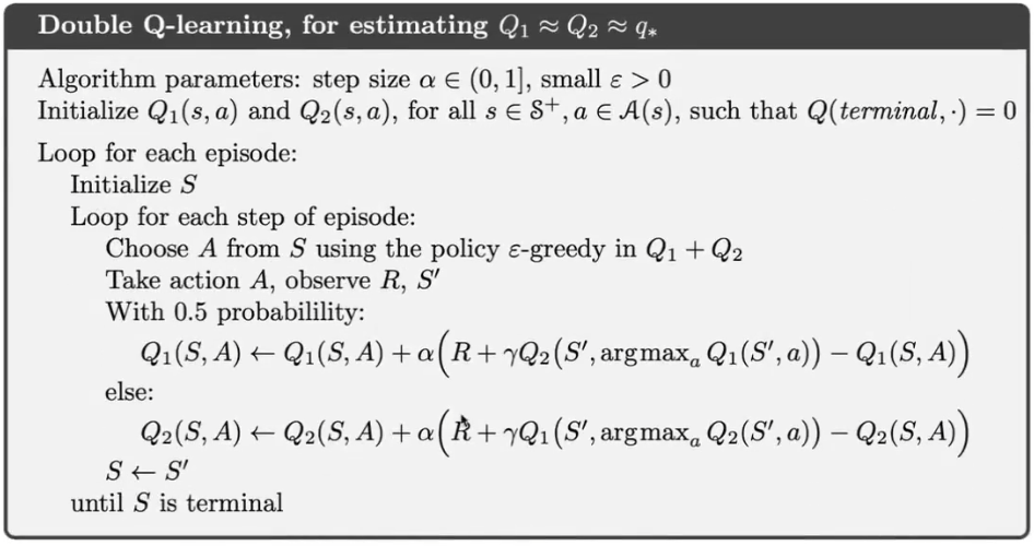
通过使用两个独立的值函数，Double-Q-Learning减轻了过估计的问题。它在每个时间步骤中随机选择一个值函数来选择动作，并使用另一个值函数来评估所选择的动作的值。这样，策略选择和值函数更新进一步解耦，减少了过估计的影响。

总结一下，Double-Q-Learning通过使用两个独立的值函数来解决Q-Learning中的过估计问题，并进一步解耦了策略选择和值函数更新。这使得Double-Q-Learning在某些情况下能够更准确地估计值函数，并更快地收敛到最优策略。

Taxi-v3

问题描述

https://gymnasium.farama.org/environments/toy_text/taxi/

This environment is part of the Toy Text environments which contains general information about the environment.

Action Space	Discrete(6)
Observation Space	Discrete(500)
import	gymnasium.make("Taxi-v3")

The Taxi Problem involves navigating to passengers in a grid world, picking them up and dropping them off at one of four locations.

Description

There are four designated pick-up and drop-off locations (Red, Green, Yellow and Blue) in the 5x5 grid world. The taxi starts off at a random square and the passenger at one of the designated locations.

The goal is move the taxi to the passenger’s location, pick up the passenger, move to the passenger’s desired destination, and drop off the passenger. Once the passenger is dropped off, the episode ends.

The player receives positive rewards for successfully dropping-off the passenger at the correct location. Negative rewards for incorrect attempts to pick-up/drop-off passenger and for each step where another reward is not received.

Map:

    +---------+
    |R: | : :G|
    | : | : : |
    | : : : : |
    | | : | : |
    |Y| : |B: |
    +---------+

From “Hierarchical Reinforcement Learning with the MAXQ Value Function Decomposition” by Tom Dietterich [1].

Action Space

The action shape is (1,) in the range {0, 5} indicating which direction to move the taxi or to pickup/drop off passengers.

• 0: Move south (down)
• 1: Move north (up)
• 2: Move east (right)
• 3: Move west (left)
• 4: Pickup passenger
• 5: Drop off passenger

Observation Space

There are 500 discrete states since there are 25 taxi positions, 5 possible locations of the passenger (including the case when the passenger is in the taxi), and 4 destination locations.

Destination on the map are represented with the first letter of the color.

Passenger locations:

• 0: Red
• 1: Green
• 2: Yellow
• 3: Blue
• 4: In taxi

Destinations:

• 0: Red
• 1: Green
• 2: Yellow
• 3: Blue

An observation is returned as an int() that encodes the corresponding state, calculated by ((taxi_row * 5 + taxi_col) * 5 + passenger_location) * 4 + destination

Note that there are 400 states that can actually be reached during an episode. The missing states correspond to situations in which the passenger is at the same location as their destination, as this typically signals the end of an episode. Four additional states can be observed right after a successful episodes, when both the passenger and the taxi are at the destination. This gives a total of 404 reachable discrete states.

Starting State

The episode starts with the player in a random state.

Rewards

• -1 per step unless other reward is triggered.
• +20 delivering passenger.
• -10 executing “pickup” and “drop-off” actions illegally.

An action that results a noop, like moving into a wall, will incur the time step penalty. Noops can be avoided by sampling the action_mask returned in info.

Episode End

The episode ends if the following happens:

• Termination: 1. The taxi drops off the passenger.
• Truncation (when using the time_limit wrapper): 1. The length of the episode is 200.

Information

step() and reset() return a dict with the following keys:

• p - transition proability for the state.
• action_mask - if actions will cause a transition to a new state.

As taxi is not stochastic, the transition probability is always 1.0. Implementing a transitional probability in line with the Dietterich paper (‘The fickle taxi task’) is a TODO.

For some cases, taking an action will have no effect on the state of the episode. In v0.25.0, info["action_mask"] contains a np.ndarray for each of the actions specifying if the action will change the state.

To sample a modifying action, use action = env.action_space.sample(info["action_mask"]) Or with a Q-value based algorithm action = np.argmax(q_values[obs, np.where(info["action_mask"] == 1)[0]]).

import gymnasium as gym

env = gym.make('Taxi-v3', render_mode='rgb_array')
env.reset()
### Output:
### (71, {'prob': 1.0, 'action_mask': array([1, 0, 1, 1, 0, 0], dtype=int8)})

Arguments

import gymnasium as gym
gym.make('Taxi-v3')

References

[1] T. G. Dietterich, “Hierarchical Reinforcement Learning with the MAXQ Value Function Decomposition,” Journal of Artificial Intelligence Research, vol. 13, pp. 227–303, Nov. 2000, doi: 10.1613/jair.639.

Version History

• v3: Map Correction + Cleaner Domain Description, v0.25.0 action masking added to the reset and step information
• v2: Disallow Taxi start location = goal location, Update Taxi observations in the rollout, Update Taxi reward threshold.
• v1: Remove (3,2) from locs, add passidx<4 check
• v0: Initial version release

准备工作

动画显示

def animate_images(images, interval=1):
    """
    以动画形式播放一组图像
    
    参数:
    images (list of numpy arrays): 包含要播放的图像的列表
    interval (float): 每个图像之间的间隔时间（秒）
    """
    # 创建一个图像对象
    fig, ax = plt.subplots()

    # 显示第一个图像
    im = ax.imshow(images[0], cmap='gray')
    plt.show()
    time.sleep(1)
    # 循环播放图像列表
    for image in images[1:]:
        # 更新图像数据
        im.set_data(image)
        # 清除当前图像
        clear_output(wait=True)
        # 显示新的图像
        display(fig)
        # 暂停一段时间
        time.sleep(1)

导入环境

import time
from collections import defaultdict

import gymnasium as gym
import numpy as np
import random

from matplotlib import pyplot as plt, animation

from tqdm.notebook import tqdm

env = gym.make('Taxi-v3', render_mode='rgb_array')

gamma = 0.95
alpha = 0.9

episode = 20000
max_steps = 100

# 计算state维度
taxi_row = 24
taxi_col = 24
passenger_location = 4
destination = 3

observation = ((taxi_row * 5 + taxi_col) * 5 + passenger_location) * 4 + destination

这是一个评价函数，用于测评训练过程中的reward函数

def evaluate(env, eval_num, policy):
    _eval_sum = 0
    for _ in range(eval_num):
        _state, _info = env.reset()
        while True:
            _action = policy(_state, _info)
            _state_next, _reward, _terminated, _truncated, _info_next = env.step(_action)
            _eval_sum += _reward
            if _terminated or _truncated:
                break
    return _eval_sum

SRASA

Q_table = np.zeros([observation, 6])

def policy_SARSA(state, info):
    eps = 0.05
    if random.random() < eps:
        return env.action_space.sample(info["action_mask"])
    else:
        array1 = np.where(info["action_mask"] == 1)[0]
        array2 = np.array(Q_table[state][array1], dtype=int)
        array3 = np.where(array2 == np.max(array2))[0]

        return array1[np.random.choice(array3)]

训练代码

sarsa_rewards = []
eval_sarsa_rewards = []
eval_iter = 100  # 每隔100次测一次
eval_num = 100

for e in tqdm(range(episode)):
    state, info = env.reset()

    sum_reward = 0    
    while True:
        action = policy_SARSA(state,info)
        state_next, reward, terminated, truncated, info_next = env.step(action)
        sum_reward += reward

        action_next = policy_SARSA(state_next, info_next)

        Q_new = reward + gamma * Q_table[state_next][action_next]
        Q_old = Q_table[state][action]

        Q_table[state][action] = alpha * (Q_new - Q_old) + Q_old

        if terminated or truncated:
            sarsa_rewards.append(sum_reward)
            break

        state = state_next
        info = info_next
        action = action_next

    if e % eval_iter == 0:
        eval_sarsa_rewards.append(evaluate(env, eval_num, policy_SARSA))

评价代码

total_rewards = 0

state, info = env.reset()
for step in range(max_steps):
    action = np.argmax(Q_table[state])
    state, reward, terminated, truncated, info_next = env.step(action)
    total_rewards += reward

    env.render()

    if terminated or truncated:
        break

env.close()

total_rewards
### Output:
### 9

Double Q-Learning

Q_table_1 = np.zeros([observation, 6])
Q_table_2 = np.zeros([observation, 6])

def policy_Double_Q_Laerning(state, info):
    eps = 0.05
    if random.random() < eps:
        return env.action_space.sample(info["action_mask"])
    else:
        action_list = np.where(info["action_mask"] == 1)[0]
        max_sum = float('-inf')
        max_index = 0
        for action in action_list:
            value = Q_table_1[state][action] + Q_table_2[state][action]
            if value > max_sum:
                max_sum = value
                max_index = action
        return max_index

def update_Q_table_1(table_1, table_2):
    Q_old = table_1[state][action]
    # action_list = np.where(info_next["action_mask"] == 1)[0]
    max_index = np.argmax(table_1[state_next])
    Q_new = reward + gamma * table_2[state_next][max_index]

    table_1[state][action] = Q_old + alpha * (Q_new - Q_old)

def update_Q_table(table_1, table_2):
    Q_old = table_1[state][action]
    action_list = np.where(info_next["action_mask"] == 1)[0]
    # max_index = np.argmax(table_1[state_next])
    max_index = 0
    max_value = float("-inf")
    for i in action_list:
        if table_1[state_next][i] > max_value:
            max_value = table_1[state_next][i]
            max_index = i

    Q_new = reward + gamma * table_2[state_next][max_index]

    table_1[state][action] = Q_old + alpha * (Q_new - Q_old)

训练代码

double_q_rewards = []
eval_double_q_rewards = []
eval_iter = 100  # 每隔100次测一次
eval_num = 100

for e in tqdm(range(episode)):
    state, info = env.reset()

    sum_reward = 0
    while True:
        action = policy_Double_Q_Laerning(state, info)
        state_next, reward, terminated, truncated, info_next = env.step(action)
        sum_reward += reward
        
        action_next = policy_Double_Q_Laerning(state_next, info_next)

        if random.random() < 0.5:
            update_Q_table(Q_table_1, Q_table_2)
        else:
            update_Q_table(Q_table_2, Q_table_1)

        if terminated or truncated:
            double_q_rewards.append(sum_reward)
            break
            
        state = state_next
        action = action_next
        info = info_next

    if e % eval_iter == 0:
        eval_double_q_rewards.append(evaluate(env, eval_num, policy_Double_Q_Laerning))

测评代码

total_rewards = 0
doule_q_frames = []

state, info = env.reset()
for step in range(max_steps):
    action = np.argmax(np.add(Q_table_1[state], Q_table_2[state]))
    state, reward, terminated, truncated, info_next = env.step(action)
    total_rewards += reward
    doule_q_frames.append(env.render())

    if terminated or truncated:
        break

env.close()

total_rewards
### Output:
### 8

动画显示

animate_images(doule_q_frames)

对比评价 Evaluation

监督学习：accuracy、precision、recall

强化学习：reward曲线

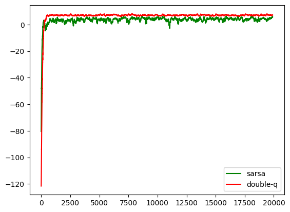
training reward

plt.plot(sarsa_rewards, c='g', label='sarsa')
plt.plot(double_q_rewards, c='r', label='double-q')

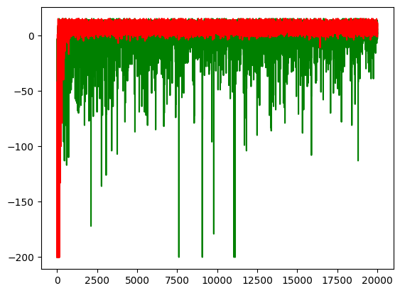
def change_scale(numbers, span=100):
    return [sum(numbers[i:i+span]) / span  for i in range(len(numbers) - span)]

plt.plot(change_scale(sarsa_rewards), c='g', label='sarsa')
plt.plot(change_scale(double_q_rewards), c='r', label='double-q')
plt.legend()

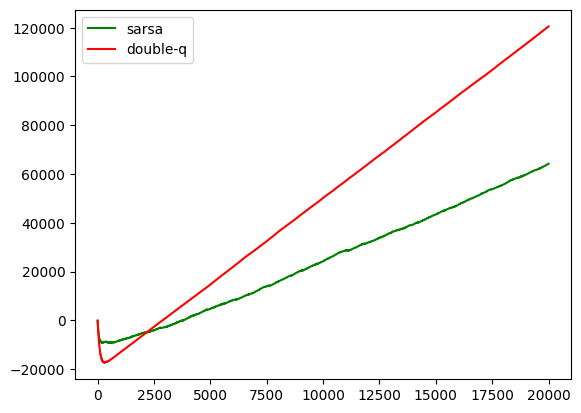
accumulated reward

# np.cumsum([1, 2, 3, 4])
# Output:
# array([1, 3, 6, 10])  # 累加

plt.plot(np.cumsum(sarsa_rewards), c='g', label='sarsa')
plt.plot(np.cumsum(double_q_rewards), c='r', label='double-q')
plt.legend()

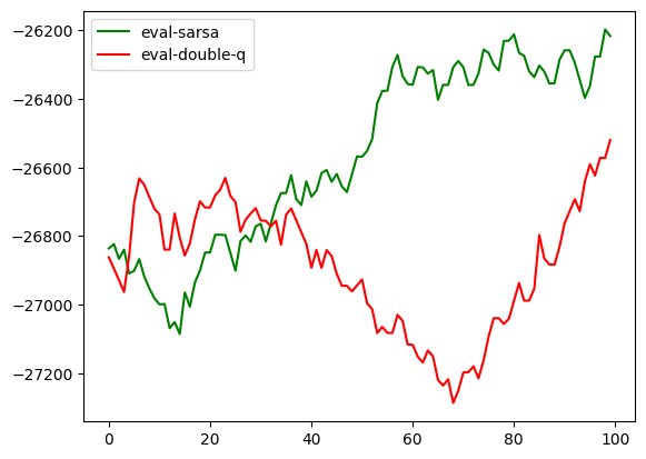
eval_reward

plt.plot(change_scale(eval_sarsa_rewards), c='g', label='eval-sarsa')
plt.plot(change_scale(eval_double_q_rewards), c='r', label='eval-double-q')
plt.legend()

‘r’, label=‘double-q’)

[外链图片转存中...(img-rzgJ2PZ9-1702483589799)]

```python
def change_scale(numbers, span=100):
    return [sum(numbers[i:i+span]) / span  for i in range(len(numbers) - span)]

plt.plot(change_scale(sarsa_rewards), c='g', label='sarsa')
plt.plot(change_scale(double_q_rewards), c='r', label='double-q')
plt.legend()

[外链图片转存中…(img-0ceMRItK-1702483589800)]

accumulated reward

# np.cumsum([1, 2, 3, 4])
# Output:
# array([1, 3, 6, 10])  # 累加

plt.plot(np.cumsum(sarsa_rewards), c='g', label='sarsa')
plt.plot(np.cumsum(double_q_rewards), c='r', label='double-q')
plt.legend()

[外链图片转存中…(img-ZGnR04MZ-1702483589800)]

eval_reward

plt.plot(change_scale(eval_sarsa_rewards), c='g', label='eval-sarsa')
plt.plot(change_scale(eval_double_q_rewards), c='r', label='eval-double-q')
plt.legend()