图像分类模型评估指南：从入门到实战，代码+图解全解析

---

导语：
在图像分类任务中，模型训练只是第一步，科学评估才是关键！本文带你手撕10+核心评估指标，用Python代码实现，附实战避坑指南，轻松拿捏模型调优！

---

一、基础指标：模型性能的“体检报告”

1. 准确率（Accuracy）

定义：全体样本中预测正确的比例，简单粗暴但可能“说谎”。
公式：

代码实现：

from sklearn.metrics import accuracy_score
y_true = [0, 1, 1, 0, 1]
y_pred = [0, 1, 0, 0, 1]
print("Accuracy:", accuracy_score(y_true, y_pred))  # 输出 0.8

2. 精确率（Precision）

定义：“宁可放过一千，不可错杀一个”——预测为正的样本中有多少是真货。
公式：

代码实现：

from sklearn.metrics import precision_score
print("Precision:", precision_score(y_true, y_pred))  # 输出 1.0（所有预测为1的都正确）

3. 召回率（Recall）

定义：“宁可错杀，不可放过”——真实的正样本有多少被捕获。
公式：

代码实现：

from sklearn.metrics import recall_score
print("Recall:", recall_score(y_true, y_pred))  # 输出 0.666（真实有3个1，正确预测2个）

4. F1-Score

定义：精确率和召回率的“调和平均数”，专治选择困难症。
公式：

代码实现：

from sklearn.metrics import f1_score
print("F1:", f1_score(y_true, y_pred))  # 输出 0.8

---

二、进阶指标：模型能力的“CT扫描”

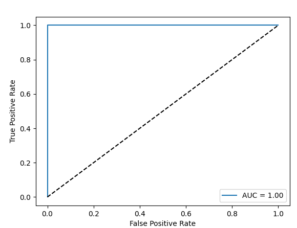
1. ROC曲线与AUC

定义：动态调整分类阈值，观察模型在不同状态下的表现。
代码实现：

import matplotlib.pyplot as plt
from sklearn.metrics import roc_curve, auc

# 生成模拟数据
y_true = [0, 1, 1, 0, 1]
y_scores = [0.1, 0.9, 0.8, 0.2, 0.7]  # 预测概率

fpr, tpr, thresholds = roc_curve(y_true, y_scores)
roc_auc = auc(fpr, tpr)

plt.plot(fpr, tpr, label=f'AUC = {roc_auc:.2f}')
plt.plot([0, 1], [0, 1], 'k--')  # 随机猜测线
plt.xlabel('False Positive Rate')
plt.ylabel('True Positive Rate')
plt.legend()
plt.show()

2. PR曲线与AP值

适用场景：正样本稀少时（如缺陷检测）比ROC更敏感。
代码实现：

from sklearn.metrics import precision_recall_curve

precision, recall, _ = precision_recall_curve(y_true, y_scores)
plt.plot(recall, precision, marker='.')
plt.xlabel('Recall')
plt.ylabel('Precision')
plt.show()

---

三、多分类场景：模型如何“雨露均沾”

1. 混淆矩阵（Confusion Matrix）

代码实现：

from sklearn.metrics import confusion_matrix
import seaborn as sns

cm = confusion_matrix(y_true, y_pred)
sns.heatmap(cm, annot=True, fmt='d')
plt.xlabel('Predicted')
plt.ylabel('True')
plt.show()

2. Top-k准确率

代码实现（以PyTorch为例）：

import torch

logits = torch.tensor([[0.2, 0.5, 0.3], [0.8, 0.1, 0.1]])  # 模型输出
targets = torch.tensor([1, 0])  # 真实标签

top1 = (logits.argmax(dim=1) == targets).float().mean()
top2 = (logits.topk(2, dim=1).indices == targets.unsqueeze(1)).any(dim=1).float().mean()

print(f"Top-1: {top1:.2f}, Top-2: {top2:.2f}")  # 输出 Top-1: 0.50, Top-2: 1.00

---

四、避坑指南：模型评估的“红灯区”

1. 类别失衡陷阱

错误做法：90%负样本的数据集，无脑预测负类准确率90%
正确操作：

# 使用加权F1
print(f1_score(y_true, y_pred, average='weighted'))

2. 阈值选择玄学

动态调整：

from sklearn.metrics import precision_recall_curve

# 找到使F1最大的阈值
precision, recall, thresholds = precision_recall_curve(y_true, y_scores)
f1_scores = 2 * precision * recall / (precision + recall)
best_idx = np.argmax(f1_scores)
print("Best threshold:", thresholds[best_idx])

---

五、实战案例：工业缺陷检测系统

场景需求

• 数据集：正常图片95%，缺陷图片5%
• 要求：召回率必须>90%，误报率<5%

代码实现关键

# 自定义评估类
class DefectEvaluator:
    def __init__(self, y_true, y_pred):
        self.tn, self.fp, self.fn, self.tp = confusion_matrix(y_true, y_pred).ravel()
    
    @property
    def recall(self):
        return self.tp / (self.tp + self.fn)
    
    @property
    def far(self):
        return self.fp / (self.fp + self.tn)
    
    def is_pass(self):
        return self.recall > 0.9 and self.far < 0.05

# 使用示例
evaluator = DefectEvaluator(y_true, y_pred)
print(f"召回率: {evaluator.recall:.2%}, 误报率: {evaluator.far:.2%}")
print("是否达标:", evaluator.is_pass())

六、特殊场景指标：当数据开始“搞事情”

1. 马修斯相关系数（MCC）

适用场景：数据严重不平衡时（如欺诈检测中99%正常交易）
公式：

代码实现：

from sklearn.metrics import matthews_corrcoef

y_true = [1, 1, 0, 0, 0, 0, 0, 0]  # 假设只有2个正样本
y_pred = [1, 0, 0, 0, 0, 0, 0, 0] 

print("MCC:", matthews_corrcoef(y_true, y_pred))  # 输出 0.33（比F1更敏感）

2. 多标签分类：Hamming Loss

代码实现：

import numpy as np
from sklearn.metrics import hamming_loss

# 多标签示例：每张图片可能属于多个类别
y_true = np.array([[1,0,1], [0,1,1], [1,1,0]])  # 3个样本，3个标签
y_pred = np.array([[1,1,1], [0,0,1], [0,1,0]])

print("Hamming Loss:", hamming_loss(y_true, y_pred))  # 输出 0.444（错误标签比例）

---

七、可视化神器：指标分析的“颜值担当”

1. 指标对比雷达图

import plotly.express as px

metrics = ['Accuracy', 'Precision', 'Recall', 'F1', 'AUC']
values = [0.85, 0.91, 0.78, 0.84, 0.88]

fig = px.line_polar(r=values, theta=metrics, line_close=True)
fig.show()

2. 动态阈值调参工具

import ipywidgets as widgets
from IPython.display import display

def update_threshold(threshold=0.5):
    y_pred = (y_scores >= threshold).astype(int)
    print(f"当前阈值: {threshold:.2f}")
    print("精确率:", precision_score(y_true, y_pred))
    print("召回率:", recall_score(y_true, y_pred))

widgets.interact(update_threshold, threshold=(0.0, 1.0, 0.05))

---

八、终极工具箱：一行代码生成报告

1. 使用Yellowbrick快速分析

from yellowbrick.classifier import ClassificationReport

model = LogisticRegression()  # 以逻辑回归为例
visualizer = ClassificationReport(model, classes=['Cat', 'Dog'])

visualizer.fit(X_train, y_train)
visualizer.score(X_test, y_test)
visualizer.show()

2. 自动化评估流水线

from sklearn.pipeline import Pipeline
from sklearn.metrics import make_scorer, fbeta_score

# 自定义F2分数（更关注召回率）
f2_scorer = make_scorer(fbeta_score, beta=2)

pipeline = Pipeline([
    ('preprocessor', StandardScaler()),
    ('classifier', RandomForestClassifier())
])

params = {'classifier__n_estimators': [100, 200]}
search = GridSearchCV(pipeline, params, scoring=f2_scorer)
search.fit(X_train, y_train)

---

九、资源大礼包：成为评估专家的秘密武器

1. 代码模板库

# 一键生成评估报告
def full_evaluation(y_true, y_pred, y_scores=None):
    print(f"准确率: {accuracy_score(y_true, y_pred):.2%}")
    print(f"精确率: {precision_score(y_true, y_pred):.2%}")
    print(f"召回率: {recall_score(y_true, y_pred):.2%}")
    print(f"F1分数: {f1_score(y_true, y_pred):.2%}")
    
    if y_scores is not None:
        print(f"AUC值: {roc_auc_score(y_true, y_scores):.2%}")
        print(f"Log Loss: {log_loss(y_true, y_scores):.3f}")

2. 推荐学习路径

学习阶段	推荐资源	难度
入门	Scikit-learn中文文档	🌟
进阶	《机器学习》周志华 第2章	🌟🌟

---

结语

通过这篇文章，我们从最基础的“体检指标”Accuracy一路升级打怪，解锁了ROC/AUC的“动态视野”，攻克了多分类的“雨露均沾”难题，最终在工业场景中完成了实战淬炼。

但请记住：模型评估从来不是终点，而是优化迭代的起点。当你下次面对99%准确率的“完美模型”时，希望你会本能地追问：“数据分布均衡吗？”、“召回率达标了吗？”、“误报成本是多少？”

那些藏在指标背后的业务逻辑，比算法本身更值得深思。现在，带上文中的代码工具箱，去大胆撕开模型的“皇帝新衣”吧——毕竟，只有经过科学评估的模型，才配得上“人工智能”这四个字。

最后，欢迎大家踊跃讨论！！！