回顾 深度学习 实验三 线性回归

需要配合深度学习 线性回归 实验三 python pytorch实现一起看

线性回归

1. 生成数据集

1. 函数：

create_toy_data(func,  # 函数
	            interval, # 范围，一个数组
			    sample_num,  # 样本数目
				noise=0.0,  # 噪音
				add_outliter=False, # 是否有异常值 
				outlier_ratio=0.001) # 异常值占比

2. 随机生成数据集，torch.rand(size)，这个函数主要生成0~1范围内的数字，要想生成指定范围，要乘以范围差值，加上范围的左值
3. 噪音：
   epsilon = torch.normal(均值，标准差，大小)
   随后y加上epsilon,生成有噪音的数据
4. 生成异常值的一种方法：让y中随机几个正常值放大5倍
5. torch.linspace(左，右，个数) # 取点
6. plt.legend() 设置图例，
   首先图像要设置label,该函数的几个参数（不全）：

参数	作用	取值
fontsize	设置图例字体大小	int or float {‘xx-small’, ‘x-small’, ‘small’, ‘medium’, ‘large’, ‘x-large’, ‘xx-large’}
frameon	去掉图例边框	False,True
edgecolor	设置图例边框颜色	blue等
facecolor	设置图例背景颜色,若无边框,参数无效	blue等

2. 模型构建

1. 线性模型定义为：
   $$f(x;w;b)=w^{T}x+b,(2.6)$$
   其中权重向量 $w\in R$和偏置 $b\in R$ 都是可学习的参数。

# X: tensor, shape=[N,D]
# y_pred: tensor, shape=[N]
# w: shape=[D,1]
# b: shape=[1]
y_pred = torch.matmul(X,w)+b # torch.matmul()两式相乘

2. torch.full()函数：

try:
    b = torch.zeros(size=[1], dtype=torch.float32)
    x = torch.full(size=[3, 1], fill_value=b)
except:
    print("我有错！！！")

运行结果：

我有错！！！

这里full_value值不能为torch.zeros(size=[1], dtype=torch.float32)

3. 模型优化

1. 转置：Tenser.t()
2. 说一下torch.mean()

代码：

y_true = torch.tensor([[-0.2], [4.9]], dtype=torch.float32)
y_pred = torch.tensor([[1.3], [2.5]], dtype=torch.float32)
error = torch.mean(torch.square(y_true - y_pred))
print("error:", error)

运行结果：

error: tensor(4.0050)

这里使用torch.mean(…).item()查看数值

y_true = torch.tensor([[-0.2], [4.9]], dtype=torch.float32)
y_pred = torch.tensor([[1.3], [2.5]], dtype=torch.float32)
error = torch.mean(torch.square(y_true - y_pred)).item()
print("error:", error)

运行结果：

error: 4.005000114440918

4. 模型优化

1. torch.inverse求方阵的逆
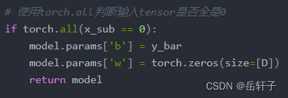
2. 使用torch.all判断输入tensor是否全是0
3. torch.subtract通过广播的方式实现矩阵减向量/
4. 这行代码的意义：

如果x_sub均等于0，那么说明X里面的值全是一个数

5. 模型训练

1. tensor.reshape()函数

# 1
X_train =  torch.rand(size=[5])
print(X_train)
X = X_train.reshape([-1, 1]) 
print(X)

运行结果：

tensor([0.4581, 0.4829, 0.3125, 0.6150, 0.2139])
tensor([[0.4581],
        [0.4829],
        [0.3125],
        [0.6150],
        [0.2139]])

# 2
X_train =  torch.rand(size=[5,2])
print(X_train)
X = X_train.reshape([-1, 1]) 
print(X)

运行结果：

tensor([[0.4581, 0.4829],
        [0.3125, 0.6150],
        [0.2139, 0.4118],
        [0.6938, 0.9693],
        [0.6178, 0.3304]])
tensor([[0.4581],
        [0.4829],
        [0.3125],
        [0.6150],
        [0.2139],
        [0.4118],
        [0.6938],
        [0.9693],
        [0.6178],
        [0.3304]])

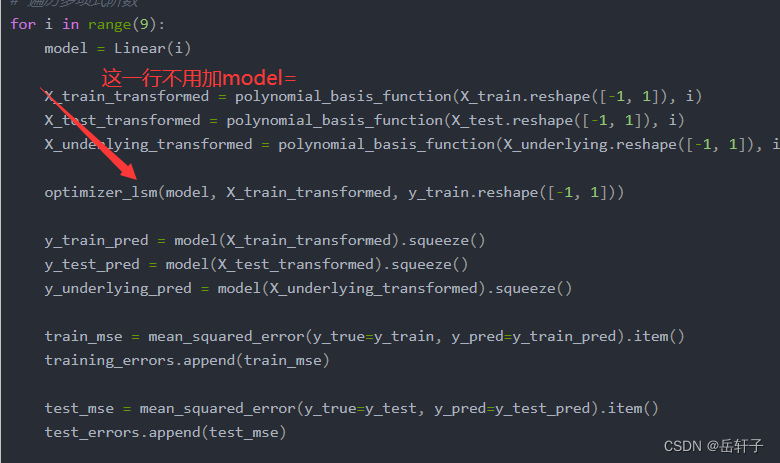
2. 注意一下：

model = optimizer_lsm(model, 
    				  X_train.reshape([-1, 1]), 
    				  y_train.reshape([-1, 1]))

这里的训练集不是直接代入的，用到了reshape()函数

2. 多项式回归

1. 数据集构建

1. $sin$ 函数

def sin(x):
    y = torch.sin(2 * math.pi * x)
    return y

2. 这行代码的意思：

plt.rcParams['figure.figsize'] = (8.0, 6.0)

设置图像显示大小，其他属性（仅展示部分）：

属性	作用	数值
axes.unicode_minus	字符显示	False,True
font.sans-serif	设置字体	例如：‘SimHei’
lines.linestyle	线条样式	例如：‘-.’
lines.linewidth	线条宽度	int
lines.color	线条颜色	‘blue’
lines.markersize	标记大小	int
xtick.labelsize	横轴字体大小	int等
xtick.major.size	x轴最大刻度	int等
axes.titlesize	子图的标题大小	int等

2. 模型构建

1. 输入：Input: [[2], [3], [4]], degree=2
   返回：Output: [[2^1, 2^2], [3^1, 3^2], [4^1, 4^2]]
2. torch.concat()元素拼接

3. 模型训练

1. enumerate()函数

for i, degree in enumerate([0, 1, 3, 8]):
    print("i:",i)
    print("degree:",degree)

输出：

i: 0
degree: 0
i: 1
degree: 1
i: 2
degree: 3
i: 3
degree: 8

2. plt.annotate()函数用于标注文字。

plt.annotate(s='str',
    xy=(x,y) ,
    xytext=(l1,l2) ,
    ...
)

s 为注释文本内容；
xy 为被注释的坐标点；
xytext 为注释文字的坐标位置；

4. 模型评估

1. 注意：
   原因：

3. Runner类

1. 代码：

class Runner(object):
    def __init__(self, model, optimizer, loss_fn, metric):
        self.model = model         # 模型
        self.optimizer = optimizer # 优化器
        self.loss_fn = loss_fn     # 损失函数   
        self.metric = metric       # 评估指标

    # 模型训练
    def train(self, train_dataset, dev_dataset=None, **kwargs):
        pass

    # 模型评价
    def evaluate(self, data_set, **kwargs):
        pass

    # 模型预测
    def predict(self, x, **kwargs):
        pass

    # 模型保存
    def save_model(self, save_path):
        pass

    # 模型加载
    def load_model(self, model_path):
        pass

如果可以的话，就记一下。

2. 缺失值分析：

# 查看各字段缺失值统计情况
data.isna().sum()

3. 四分位数处理异常值

# 四分位处理异常值
num_features = data.select_dtypes(exclude=['object','bool']).columns.tolist()

for feature in num_features:
    if feature == 'CHAS':
        continue

    Q1 = data[feature].quantile(q=0.25) # 下四分位
    Q3 = data[feature].quantile(q=0.75) # 上四分位

    IQR = Q3-Q1
    top = Q3+1.5*IQR
    bot = Q1-1.5*IQR
    values = data[feature].values
    values[values>top] = top
    values[values<bot] = bot
    data[feature] = values.astype(data[feature].dtypes)

# 再次查看箱线图，异常值已被临界值替换（数据量较多或本身异常值较少时，箱线图展示会不容易体现出来）
boxplot(data, 'ml-vis6.pdf')

这里说一下select_dtypes()和astype()

1. select_dtypes()根据它们的数据类型选择列
2. astype()进行类型转换

求四分位：

• data[feature].quantile(q=0.25) # 下四分位
• data[feature].quantile(q=0.75) # 上四分位

另一种：

• np.percentile(数据, 25, interpolation=‘linear’) # 下四分位
• np.percentile(数据, 75, interpolation=‘linear’) # 上四分位

---

这里都是我自己总结的小笔记，有点乱

如果对你有帮助的话，求求你给我一个赞吧！！！

如有错误与建议，望告知！！！（将于下篇文章更正）
请多多关注我！！！谢谢！！！