


前几期我们介绍了MODIS和LANDSAT8遥感影像的MDVI时间序列,其他数据也与此类似,大家根据实际情况修改即可。本期我们介绍Sentinel-2 Level-2A数据在时间序列方面的研究。
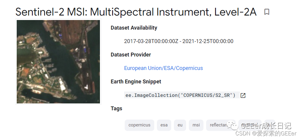
COPERNICUS/S2_SR
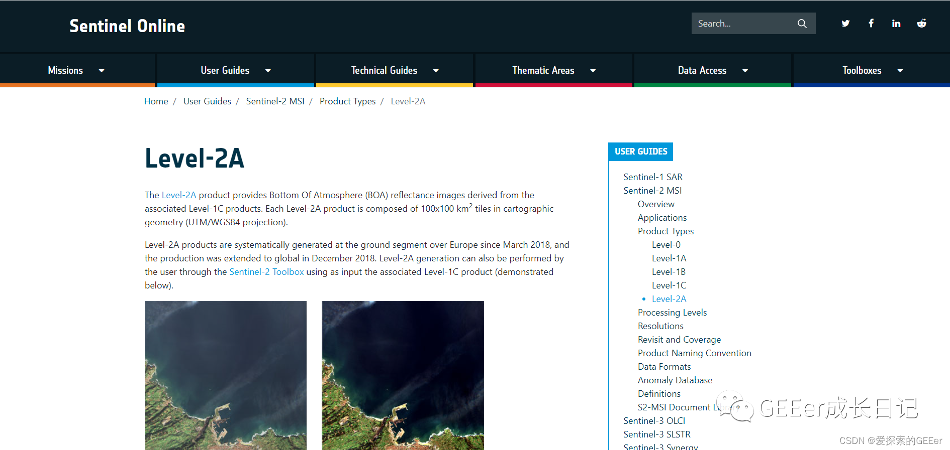
如果想深入了解这两个数据集,可以登录:
https://sentinel.esa.int/web/sentinel/user-guides/sentinel-2-msi/product-types/level-2a
European Union/ESA/Copernicus
https://sentinel.esa.int/web/sentinel/user-guides/sentinel-2-msi/resolutions/radiometric
辐射分辨率介绍
GEE官方介绍:Sentinel-2 is a wide-swath, high-resolution, multi-spectral imaging mission supporting Copernicus Land Monitoring studies, including the monitoring of vegetation, soil and water cover, as well as observation of inland waterways and coastal areas.
The Sentinel-2 L2 data are downloaded from scihub. They were computed by running sen2cor. WARNING: ESA did not produce L2 data for all L1 assets, and earlier L2 coverage is not global.
The assets contain 12 UINT16 spectral bands representing SR scaled by 10000 (unlike in L1 data, there is no B10). There are also several more L2-specific bands (see band list for details). See the Sentinel-2 User Handbook for details. In addition, three QA bands are present where one (QA60) is a bitmask band with cloud mask information. For more details, see the full explanation of how cloud masks are computed.
EE asset ids for Sentinel-2 L2 assets have the following format: COPERNICUS/S2_SR/20151128T002653_20151128T102149_T56MNN. Here the first numeric part represents the sensing date and time, the second numeric part represents the product generation date and time, and the final 6-character string is a unique granule identifier indicating its UTM grid reference (see MGRS).
Clouds can be removed by using COPERNICUS/S2_CLOUD_PROBABILITY. See this tutorial explaining how to apply the cloud mask.
分辨率:10m
熟悉的朋友应该都熟悉

Landsat8的NDVI计算是通过4、5波段,而哨兵2号数据的NDVI计算是通过4、8波段。
继续引用大佬的总结:
NDVI = (近红外波段 - 红波段) / (近红外波段 + 红波段)
针对每种卫星的波段,选用的波段都有所不同,公式如下:
Landsat8: NDVI = (band5 - band4) / (band5 + band4)
Sentinel2: NDVI = (band8 - band4) / (band8 + band4)
Modis: NDVI = (band2 - band1) / (band2 + band1)
ETM/TM: NDVI = (band4 - band3) / (band4 + band3)
AVHRR: NDVI = (CH2 - CH1) / (CH2 + CH1)
因为哨兵系列数据分辨率高,我们在研究过程中考虑的分辨率还是500。话不多说,开始~
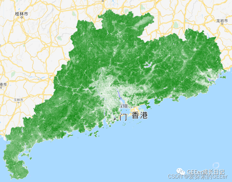
//还是老样子哈,以广东省2020年为目标
var geometry = ee.FeatureCollection('users/ZhengkunWang/guangdongsheng')
Map.centerObject(geometry,7)
//还是原来的配方,还是原来的调色板
var colorizedVis = {
min: -0.8,
max: 0.8,
palette: ['blue', 'white', 'green'],
};
//使用QA波段去云
function maskS2clouds(image) {
var qa = image.select('QA60');
// Bits 10 and 11 are clouds and cirrus, respectively.
var cloudBitMask = 1 << 10;
var cirrusBitMask = 1 << 11;
// Both flags should be set to zero, indicating clear conditions.
var mask = qa.bitwiseAnd(cloudBitMask).eq(0)
.and(qa.bitwiseAnd(cirrusBitMask).eq(0));
return image.updateMask(mask).divide(10000).set(image.toDictionary(image.propertyNames()));
}
//特别注意的是,在数学变换之后,保持原始影像的属性,所以这里.set(image.toDictionary(image.propertyNames()));就是这个意思
//sentinel2 and geometry
var S2_COL = ee.ImageCollection("COPERNICUS/S2")
.filterDate("2020-01-01", "2020-12-31")
.filter(ee.Filter.lt('CLOUDY_PIXEL_PERCENTAGE',20))
.filterBounds(geometry)
.map(maskS2clouds)
.map(function(image){
var ndvi = image.normalizedDifference(["B8","B4"]).rename('NDVI')
return image.addBands(ndvi)
})
.select('NDVI');
print(S2_COL)
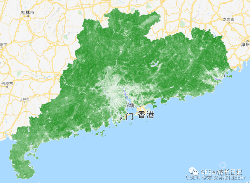
Map.addLayer(S2_COL.mean().clip(geometry), colorizedVis, 'col');
var S2_chart = ui.Chart.image.series({
imageCollection: S2_COL.select('NDVI'),
region: geometry,
reducer: ee.Reducer.mean(),
scale: 500
}).setOptions({
interpolateNulls: true,
lineWidth: 2,
title: 'NDVI Time Seires',
vAxis: {title: 'NDVI'},
hAxis: {title: 'Date'},
trendlines: { 0: {title: 'NDVI_trend',type:'linear', showR2: true, color:'red', visibleInLegend: true}}
});
print(S2_chart);这次我们一气呵成
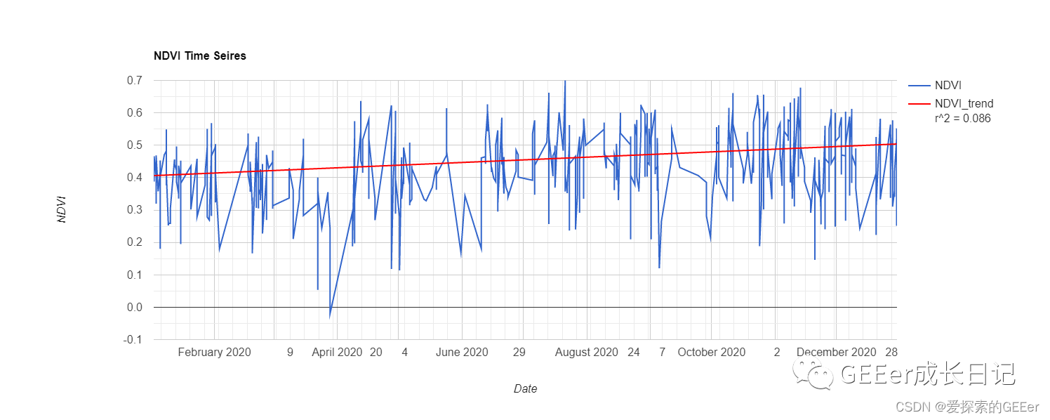
观察这个时间序列可以发现,同一天因为有好多轨道影像的原因,导致同一天有很多不同的值,所以我们需要进行日平均或月平均计算。今天我们先介绍月平均的时间序列分析。
var geometry = ee.FeatureCollection('users/ZhengkunWang/guangdongsheng')
Map.centerObject(geometry,6)

var colorizedVis = {
  min: -0.8,
  max: 0.8,
  palette: ['blue', 'white', 'green'],
};

//使用QA波段去云
function maskS2clouds(image) {
  var qa = image.select('QA60');
  // Bits 10 and 11 are clouds and cirrus, respectively.
  var cloudBitMask = 1 << 10;
  var cirrusBitMask = 1 << 11;
  // Both flags should be set to zero, indicating clear conditions.
  var mask = qa.bitwiseAnd(cloudBitMask).eq(0)
      .and(qa.bitwiseAnd(cirrusBitMask).eq(0));
  return image.updateMask(mask).divide(10000).set(image.toDictionary(image.propertyNames()));
}
var S2 = ee.ImageCollection('COPERNICUS/S2')
.filterDate('2020-01-01', '2020-12-31')
.filterBounds(geometry)
.filter(ee.Filter.lt('CLOUDY_PIXEL_PERCENTAGE', 20))
.map(maskS2clouds);
var addNDVI = function(image) {
return image.addBands(image.normalizedDifference(['B8', 'B4']).rename('NDVI'));
};
// Add NDVI band to image collection
var S2 = S2.map(addNDVI);
var NDVI = S2.select(['NDVI']);
print(NDVI);
var NDVImed = NDVI.median();
Map.addLayer(NDVImed.clip(geometry), colorizedVis, 'NDVI image');


var years = ee.List.sequence(2020, 2020);
var months = ee.List.sequence(1, 12);
var S2_monthlymeanNDVI =  ee.ImageCollection.fromImages(
  years.map(function (y) {
    return months.map(function(m) {
    return NDVI.filter(ee.Filter.calendarRange(y,y, 'year')).filter(ee.Filter.calendarRange(m, m, 'month')).mean().set('year', y).set('month', m).set('system:time_start', ee.Date.fromYMD(y, m, 1));
    });
  }).flatten()
);
// Create a monthly time series chart.
var plotNDVI = ui.Chart.image.seriesByRegion(S2_monthlymeanNDVI, geometry,ee.Reducer.mean(),
'NDVI',500,'system:time_start')
              .setChartType('LineChart').setOptions({
                interpolateNulls: true,
                title: 'NDVI Monthly time series',
                hAxis: {title: 'Date'},
                vAxis: {title: 'NDVI',viewWindowMode: 'explicit', viewWindow: {max: 0.7,min: 0.3,},gridlines: {count: 10,}},
                trendlines: { 0: {title: 'NDVI_trend',type:'linear', showR2: true,  color:'red', visibleInLegend: true}}});
// Display.
print(plotNDVI);
可能是影像太多了,算了好几分钟,终于搞定:
结果如图:
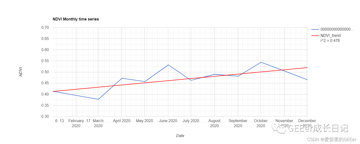
看完时间序列的话,拟合性还可以,但是全年一直增长?这合适吗?而且日期序号也有错误,小编还在找问题,如果有大神看出来的话,可以指点我一下下。
更多精彩内容请关注:


 821
821

 被折叠的 条评论
为什么被折叠?
被折叠的 条评论
为什么被折叠?
 到【灌水乐园】发言


