


10.12学习笔记 - 决策树
学习了分类和回归问题下的决策树模型,手写决策树结构
一、决策树处理分类问题 - 鸢尾花
1.数据处理&划分数据集
# 引入包

from sklearn.tree import DecisionTreeClassifier
from sklearn.tree import DecisionTreeRegressor
from sklearn.tree import plot_tree

from sklearn.datasets import load_boston
from sklearn.datasets import load_iris

from sklearn.model_selection import train_test_split

import numpy as np
from matplotlib import pyplot as plt

# 加载数据集
X, y = load_iris(return_X_y=True)

# 切分数据集
X_train, X_test, y_train, y_test =train_test_split(X,y,test_size=0.15,random_state=1)

# 构建分类模型
dtc = DecisionTreeClassifier(max_depth=2)
# 这里默认为gini,以下两种情况都会阐述

# 模型评估
score = dtc.score(X=X_test, y=y_test)
# output: 0.9565217391304348

# 绘制决策树
plot_tree(dtc)
2.计算信息熵&构建二叉树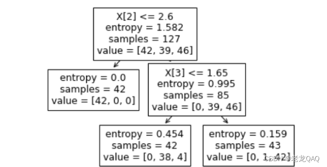
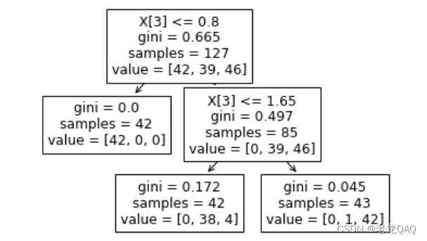
上图为sklearn中plot_tree绘制出的决策树,DecisionTreeClassifier()参数为criterion="entropy"
根节点内容解释:
- x[3] <= 0.8 以x的第三个特征是否小于0.8为判断标准
- entropy —> 信息熵 —>代表信息混乱程度
- samples = 127 ===》有127个样本
- value = [42,39,46] 第一类有42个,第二类有39个…
"""
    计算训练集的熵

"""
samples = np.array([42, 39, 46])
p = samples / samples.sum()
entropy = -(p* np.log2(p)).sum()
entropy
# outputing: 1.5816621019614714
"""
遍历每个特征及其分割值
寻找下降最大的分割点

"""
X_train.shape
for feaure_idx in range(4):

    print("当前分割特征为", feaure_idx)

    for value in set(X_train[:, feaure_idx]):  # set 去重减少数据量
        print("分割值:", value)

        left_idx = X_train[:, feaure_idx] <= value
        right_idx = X_train[:, feaure_idx] > value

        X_left = X_train[left_idx]
        X_right = X_train[right_idx]

        print("向左走", X_left)
        print("向右走", X_right)

        break # 跳出当前循环

    break
- 当数据量非常大、任务非常复杂时,观察内部细节可以通过break来打印第一个内(外)层循环
(1).计算信息熵
如何确定信息熵降低最快呢 —> 遍历每一个特征,比较遍历后的左右子树加权平均值
def get_entrepy(y):
    # 判断value如果是最大则没有右子树
    if len(y) == 0:
        return 0
    samples = np.array([y.tolist().count(idx) for idx in range(3)])
    p = samples /samples.sum() + 1e-6
    entropy = -(p * np.log2(p)).sum()
    return entropy
X_train.shape
for feaure_idx in range(4):

    print("当前分割特征为", feaure_idx)

    for value in set(X_train[:, feaure_idx]):  # set 去重减少数据量
        print("分割值:", value)

        left_idx = X_train[:, feaure_idx] <= value
        right_idx = X_train[:, feaure_idx] > value

        #求信息熵:计算每一类的概率,然后把每一类的概率相乘再相加再取负号

        # 求左边样本个数
        n_left = len(left_idx)
        n_right = len(right_idx)
        if n_left == 0 or n_right == 0:
            continue

        # 左
        X_left = X_train[left_idx]
        y_left = y_train[left_idx]

        # 左熵
        """
        print("左侧熵:", y_left)
        temp = {0:0, 1:0, 2:0} # 初始化一个temp 第0类为0个,第1类为0个,第2类为0个
        for ele in y_left: # 遍历,是哪一类哪一类就加1
            temp[ele] += 1
        print(temp)

        samples = list(temp.values())
        print(samples)

        """
        entropy_left = get_entrepy(y_left)
        print(entropy_left)

        # print([y_left.tolist().count(idx) for idx in range(3)])

        # 右
        X_right = X_train[right_idx]
        y_right = y_train[right_idx]

        # print("右侧熵", y_right)

        entropy_right = get_entrepy(y_right)
        print(entropy_right)

        # print("向左走", X_left)
        # print("向右走", X_right)

        # 加权平均
        entropy = n_left / (n_left + n_right) * entropy_left + n_right / (
            n_left + n_right) * entropy_right
        print(entropy)
            # 另一种写法
        print(np.average(a = np.array([entropy_left,entropy_right]),weights = np.array([n_left,n_right])))

        break

    break
"""output

当前分割特征为 0
分割值: 4.8
3.8420441376530785e-05
1.5562814756042398
0.7781599480228082
0.7781599480228082
"""
判断哪个熵减最大,思路是计算所有分出值的熵的最小值
#              特征编号       当前分割值           entropy
best_split = {"feature_idx":0,"feature_value":0,"entropy":np.inf}

for feaure_idx in range(4):

    # print("当前分割特征为", feaure_idx)

    for value in set(X_train[:, feaure_idx]):  # set 去重减少数据量
        # print("分割值:", value)

        left_idx = X_train[:, feaure_idx] <= value
        right_idx = X_train[:, feaure_idx] > value

        #求信息熵:计算每一类的概率,然后把每一类的概率相乘再相加再取负号

        # 求左边样本个数 这里不能用len 因为right_idx里面是True和False,长度一样
        n_left = sum(left_idx)
        n_right = sum(right_idx)

        # 左
        X_left = X_train[left_idx]
        y_left = y_train[left_idx]

        # 左熵
        """
        print("左侧熵:", y_left)
        temp = {0:0, 1:0, 2:0} # 初始化一个temp 第0类为0个,第1类为0个,第2类为0个
        for ele in y_left: # 遍历,是哪一类哪一类就加1
            temp[ele] += 1
        print(temp)

        samples = list(temp.values())
        print(samples)

        """
        entropy_left = get_entrepy(y_left)
        # print(entropy_left)

        # print([y_left.tolist().count(idx) for idx in range(3)])

        # 右
        X_right = X_train[right_idx]
        y_right = y_train[right_idx]

        # print("右侧熵", y_right)

        entropy_right = get_entrepy(y_right)
        # print(entropy_right)

        # print("向左走", X_left)
        # print("向右走", X_right)

        # 加权平均
        entropy = n_left / (n_left + n_right) * entropy_left + n_right / (n_left + n_right) * entropy_right
        # print(entropy)
        # 另一种写法
        # print(np.average(a = np.array([entropy_left,entropy_right]),weights = np.array([n_left,n_right])))

        # 判断是否为最佳 - 野蛮计算 穷举思想
        if entropy < best_split["entropy"]:
            best_split["feature_idx"] = feaure_idx
            best_split['feature_value'] = value
            best_split["entropy"] = entropy
注意:np.inf 代表无穷大(infinity)
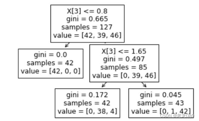
输出计算结果best_split:
best_split
# output:{'feature_idx': 2, 'feature_value': 1.9, 'entropy': 0.666038791145047}
- 这里发现与sklearn中feature_value有差距,接着完善
values = list(set(X_train[:,2]))  # X_train[:,2]行都要第二列
values.sort()
values
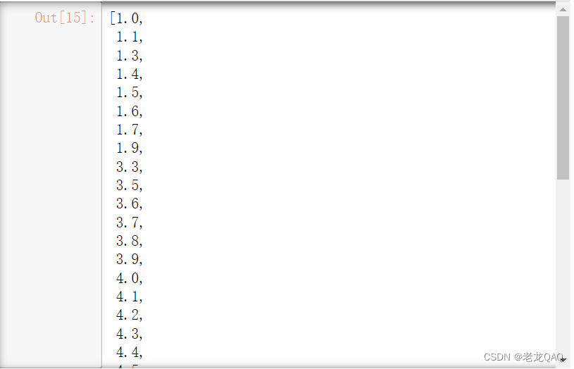
上图为计算结果,可以发现这里遍历的是离散值,所以feature_value会从上面的数字中产生,而sklearn中将数据视为连续数据所以将 (1.9+3.3)/ 2 = 2.6 做为分割值,鲁棒性会更高
4.基尼系数
- Q:为什么工程中都使用基尼系数呢?
-
基尼系数 gini = P*(1-P)
-
entropy = -P(logP)
(1-P)和(logP)都是大于零的减函数,从逻辑上讲都是一样的,但是(1-P)计算代价很低,所以不妨用(1-P)代替(logP)
-
(1).计算基尼系数
def get_gini(y):
    """
        根据标签,计算 gini 系数
    """

    samples = np.array([y.tolist().count(idx) for idx in range(3)])

    print(samples)
    p = samples / samples.sum()

    gini = (p * (1-p)).sum()

    return gini
二、回归问题 -波士顿房价预测
1.划分数据集
X,y = load_boston(return_X_y=True)

X_train, X_test, y_train, y_test =train_test_split(X,y,test_size=0.12,random_state=1)

dtr = DecisionTreeRegressor(max_depth=2)

dtr.fit(X=X_train,y=y_train)

plot_tree(dtr)
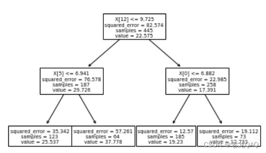
这里的value其实就是均值
y_train.mean()
# output:22.574831460674158
- 回归问题怎么求信息熵 (一堆连续数据怎么衡量混乱程度 ) ==》方差
y_train.var()
# output:82.57397328620124
这里的mse是假mse 其实就是方差
"""
    穷举思想

    遍历每个特征及其分割值
    寻找方差下降最快的分割点

"""

#              特征编号       当前分割值           entropy
best_split = {"feature_idx":0,"feature_value":0,"mse":np.inf}

for feaure_idx in range(13): # 13 个特征

    # print("当前分割特征为", feaure_idx)

    for value in set(X_train[:, feaure_idx]):  # set 去重减少数据量
        # print("分割值:", value)

        left_idx = X_train[:, feaure_idx] <= value
        right_idx = X_train[:, feaure_idx] > value

        #求信息熵:计算每一类的概率,然后把每一类的概率相乘再相加再取负号

        # 求左边样本个数 这里不能用len 因为right_idx里面是True和False,长度一样
        n_left = sum(left_idx)
        n_right = sum(right_idx)

        if n_right == 0:
            continue

        # 左
        X_left = X_train[left_idx]
        y_left = y_train[left_idx]

        # 左熵
        """
        print("左侧熵:", y_left)
        temp = {0:0, 1:0, 2:0} # 初始化一个temp 第0类为0个,第1类为0个,第2类为0个
        for ele in y_left: # 遍历,是哪一类哪一类就加1
            temp[ele] += 1
        print(temp)

        samples = list(temp.values())
        print(samples)

        """
        mse_left = y_left.var()
        # print(entropy_left)

        # print([y_left.tolist().count(idx) for idx in range(3)])

        # 右
        X_right = X_train[right_idx]
        y_right = y_train[right_idx]

        # print("右侧熵", y_right)

        mse_right = y_right.var()
        # print(entropy_right)

        # print("向左走", X_left)
        # print("向右走", X_right)

        # 加权平均
        mse = n_left / (n_left + n_right) * mse_left + n_right / (n_left + n_right) * mse_right
        # print(entropy)
        # 另一种写法
        # print(np.average(a = np.array([entropy_left,entropy_right]),weights = np.array([n_left,n_right])))

        # 判断是否为最佳 - 野蛮计算 穷举思想
        if mse < best_split["mse"]:
            best_split["feature_idx"] = feaure_idx
            best_split['feature_value'] = value
            best_split["mse"] = mse
best_split # 同理 (71+74) / 2 = 72.5
# output:{'feature_idx': 12, 'feature_value': 9.71, 'mse': 45.50584908896213}
查看feature_value
sorted(X_train[:,12])


 7161
7161

 被折叠的 条评论
为什么被折叠?
被折叠的 条评论
为什么被折叠?
 到【灌水乐园】发言


