基于tensorflow的咖啡豆识别

• 🍨 本文为🔗365天深度学习训练营 中的学习记录博客
• 🍖 原作者：K同学啊

一、前期工作

1. 设置GPU

import tensorflow as tf

gpus = tf.config.list_physical_devices("GPU")

if gpus:
    tf.config.experimental.set_memory_growth(gpus[0], True)  #设置GPU显存用量按需使用
    tf.config.set_visible_devices([gpus[0]],"GPU")
    print("GPU is available")

2. 导入数据

from tensorflow       import keras
from tensorflow.keras import layers,models
import numpy             as np
import matplotlib.pyplot as plt
import os,PIL,pathlib

data_dir = "F:/host/Data/咖啡豆识别数据/"
data_dir = pathlib.Path(data_dir)

image_count = len(list(data_dir.glob('*/*.png')))

print("图片总数为：",image_count)

二、数据预处理

1. 加载数据

使用image_dataset_from_directory方法将磁盘中的数据加载到tf.data.Dataset中

batch_size = 8
img_height = 224
img_width = 224

train_ds = tf.keras.preprocessing.image_dataset_from_directory(
    data_dir,
    validation_split=0.2,
    subset="training",
    seed=123,
    image_size=(img_height, img_width),
    batch_size=batch_size)

val_ds = tf.keras.preprocessing.image_dataset_from_directory(
    data_dir,
    validation_split=0.1,
    subset="validation",
    seed=123,
    image_size=(img_height, img_width),
    batch_size=batch_size)

class_names = train_ds.class_names
print(class_names)

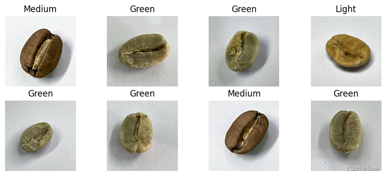
2. 可视化数据

plt.figure(figsize=(10, 4))  # 图形的宽为10高为5

for images, labels in train_ds.take(1):
    for i in range(8):
        
        ax = plt.subplot(2, 4, i + 1)  

        plt.imshow(images[i].numpy().astype("uint8"))
        plt.title(class_names[labels[i]])
        
        plt.axis("off")

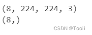
for image_batch, labels_batch in train_ds:
    print(image_batch.shape)
    print(labels_batch.shape)
    break

3. 配置数据集

• shuffle() ：打乱数据，关于此函数的详细介绍可以参考：https://zhuanlan.zhihu.com/p/42417456
• prefetch() ：预取数据，加速运行，其详细介绍可以参考我前两篇文章，里面都有讲解。
• cache() ：将数据集缓存到内存当中，加速运行

AUTOTUNE = tf.data.AUTOTUNE

train_ds = train_ds.cache().shuffle(1000).prefetch(buffer_size=AUTOTUNE)
val_ds   = val_ds.cache().prefetch(buffer_size=AUTOTUNE)

normalization_layer = layers.experimental.preprocessing.Rescaling(1./255)

train_ds = train_ds.map(lambda x, y: (normalization_layer(x), y))
val_ds   = val_ds.map(lambda x, y: (normalization_layer(x), y)) 

image_batch, labels_batch = next(iter(val_ds))
first_image = image_batch[0]

# 查看归一化后的数据
print(np.min(first_image), np.max(first_image))

三、构建VGG-16网络

from tensorflow.keras import layers, models, Input
from tensorflow.keras.models import Model
from tensorflow.keras.layers import Conv2D, MaxPooling2D, Dense, Flatten, Dropout

def VGG16(nb_classes, input_shape):
    # 输入层
    input_tensor = Input(shape=input_shape)
    # 卷积层1
    x = Conv2D(64, (3,3), activation='relu', padding='same',name='block1_conv1')(input_tensor)
    x = Conv2D(64, (3,3), activation='relu', padding='same',name='block1_conv2')(x)
    x = MaxPooling2D((2,2), strides=(2,2), name = 'block1_pool')(x)
    # 卷积层2
    x = Conv2D(128, (3,3), activation='relu', padding='same',name='block2_conv1')(x)
    x = Conv2D(128, (3,3), activation='relu', padding='same',name='block2_conv2')(x)
    x = MaxPooling2D((2,2), strides=(2,2), name = 'block2_pool')(x)
    # 卷积层3
    x = Conv2D(256, (3,3), activation='relu', padding='same',name='block3_conv1')(x)
    x = Conv2D(256, (3,3), activation='relu', padding='same',name='block3_conv2')(x)
    x = Conv2D(256, (3,3), activation='relu', padding='same',name='block3_conv3')(x)
    x = MaxPooling2D((2,2), strides=(2,2), name = 'block3_pool')(x)
    # 卷积层4
    x = Conv2D(512, (3,3), activation='relu', padding='same',name='block4_conv1')(x)
    x = Conv2D(512, (3,3), activation='relu', padding='same',name='block4_conv2')(x)
    x = Conv2D(512, (3,3), activation='relu', padding='same',name='block4_conv3')(x)
    x = MaxPooling2D((2,2), strides=(2,2), name = 'block4_pool')(x)
    # 卷积层5
    x = Conv2D(512, (3,3), activation='relu', padding='same',name='block5_conv1')(x)
    x = Conv2D(512, (3,3), activation='relu', padding='same',name='block5_conv2')(x)
    x = Conv2D(512, (3,3), activation='relu', padding='same',name='block5_conv3')(x)
    x = MaxPooling2D((2,2), strides=(2,2), name = 'block5_pool')(x)
    # 展平层
    x = Flatten()(x)
    # 全连接层1
    x = Dense(4096, activation='relu',name='fc1')(x)
    # 全连接层2
    x = Dense(4096, activation='relu',name='fc2')(x)
    # 输出层
    output_tensor = Dense(nb_classes, activation='softmax',name='predictions')(x)
    # 创建模型
    model = Model(input_tensor, output_tensor)
    return model

# 创建模型
model=VGG16(len(class_names), (img_width, img_height, 3))

# 打印模型结构
model.summary()

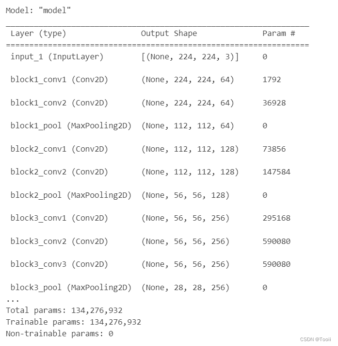
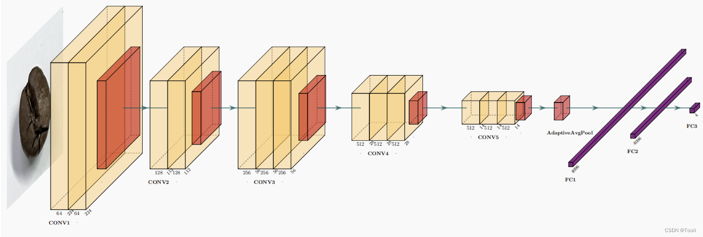
3. 网络结构图

关于卷积的相关知识可以参考文章：https://mtyjkh.blog.csdn.net/article/details/114278995

结构说明：

• 13个卷积层（Convolutional Layer），分别用blockX_convX表示
• 3个全连接层（Fully connected Layer），分别用fcX与predictions表示
• 5个池化层（Pool layer），分别用blockX_pool表示

VGG-16包含了16个隐藏层（13个卷积层和3个全连接层），故称为VGG-16

四、编译

在准备对模型进行训练之前，还需要再对其进行一些设置。以下内容是在模型的编译步骤中添加的：

• 损失函数（loss）：用于衡量模型在训练期间的准确率。
• 优化器（optimizer）：决定模型如何根据其看到的数据和自身的损失函数进行更新。
• 指标（metrics）：用于监控训练和测试步骤。以下示例使用了准确率，即被正确分类的图像的比率。

# 设置初始学习率
initial_learning_rate = 1e-4

lr_schedule = tf.keras.optimizers.schedules.ExponentialDecay(
        initial_learning_rate, 
        decay_steps=30,      # 敲黑板！！！这里是指 steps，不是指epochs
        decay_rate=0.92,     # lr经过一次衰减就会变成 decay_rate*lr
        staircase=True)

# 设置优化器
opt = tf.keras.optimizers.Adam(learning_rate=initial_learning_rate)

model.compile(optimizer=opt,
              loss=tf.keras.losses.SparseCategoricalCrossentropy(from_logits=True),
              metrics=['accuracy'])

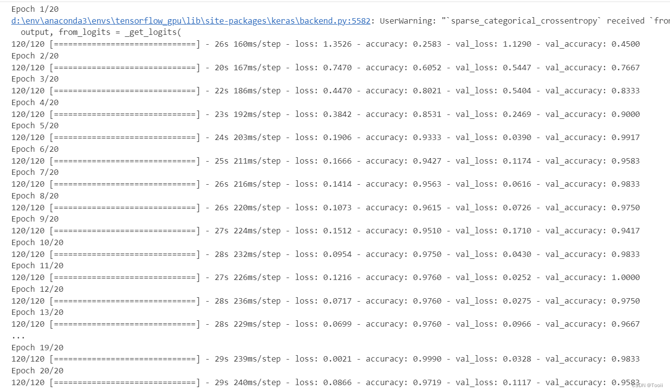
五、训练模型

epochs = 20

history = model.fit(
    train_ds,
    validation_data=val_ds,
    epochs=epochs
)

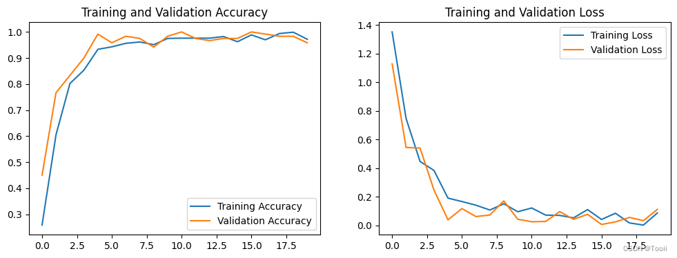
六、可视化结果

acc = history.history['accuracy']
val_acc = history.history['val_accuracy']

loss = history.history['loss']
val_loss = history.history['val_loss']

epochs_range = range(epochs)

plt.figure(figsize=(12, 4))
plt.subplot(1, 2, 1)
plt.plot(epochs_range, acc, label='Training Accuracy')
plt.plot(epochs_range, val_acc, label='Validation Accuracy')
plt.legend(loc='lower right')
plt.title('Training and Validation Accuracy')

plt.subplot(1, 2, 2)
plt.plot(epochs_range, loss, label='Training Loss')
plt.plot(epochs_range, val_loss, label='Validation Loss')
plt.legend(loc='upper right')
plt.title('Training and Validation Loss')
plt.show()

七、个人小结

在本次咖啡豆识别项目中，我们通过设置GPU、导入并预处理数据、构建深度学习模型，以及对模型进行训练和评估，实现了对咖啡豆图像的自动识别。整个过程涵盖了数据加载与可视化、数据集配置、模型构建与优化等关键步骤，最终显著提升了图像分类的准确性，同时也加深了我们对深度学习技术的实践理解。