


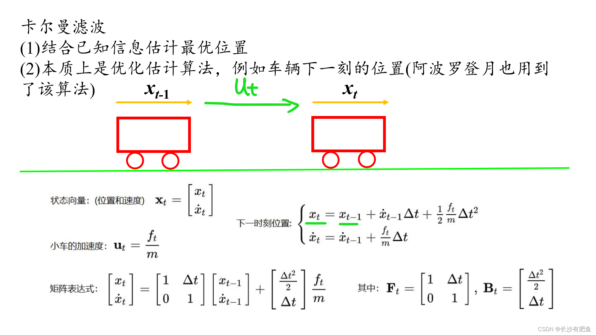
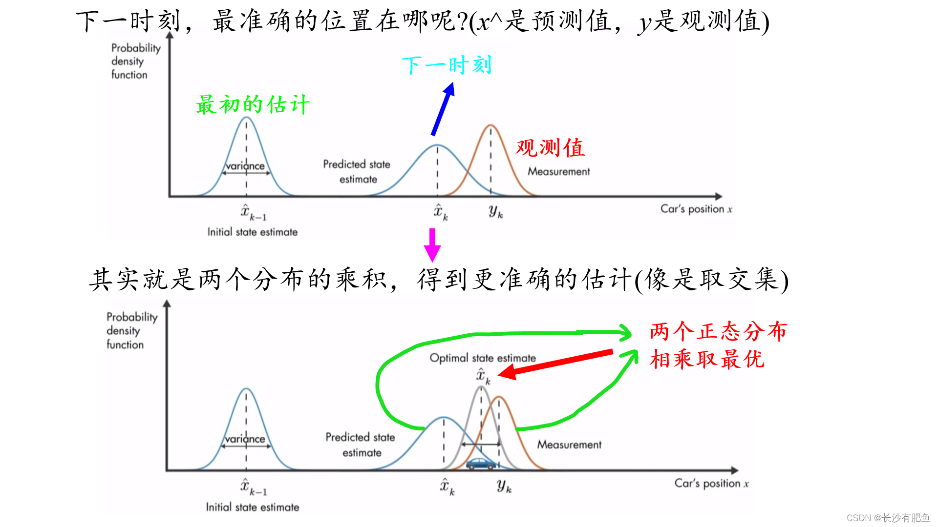
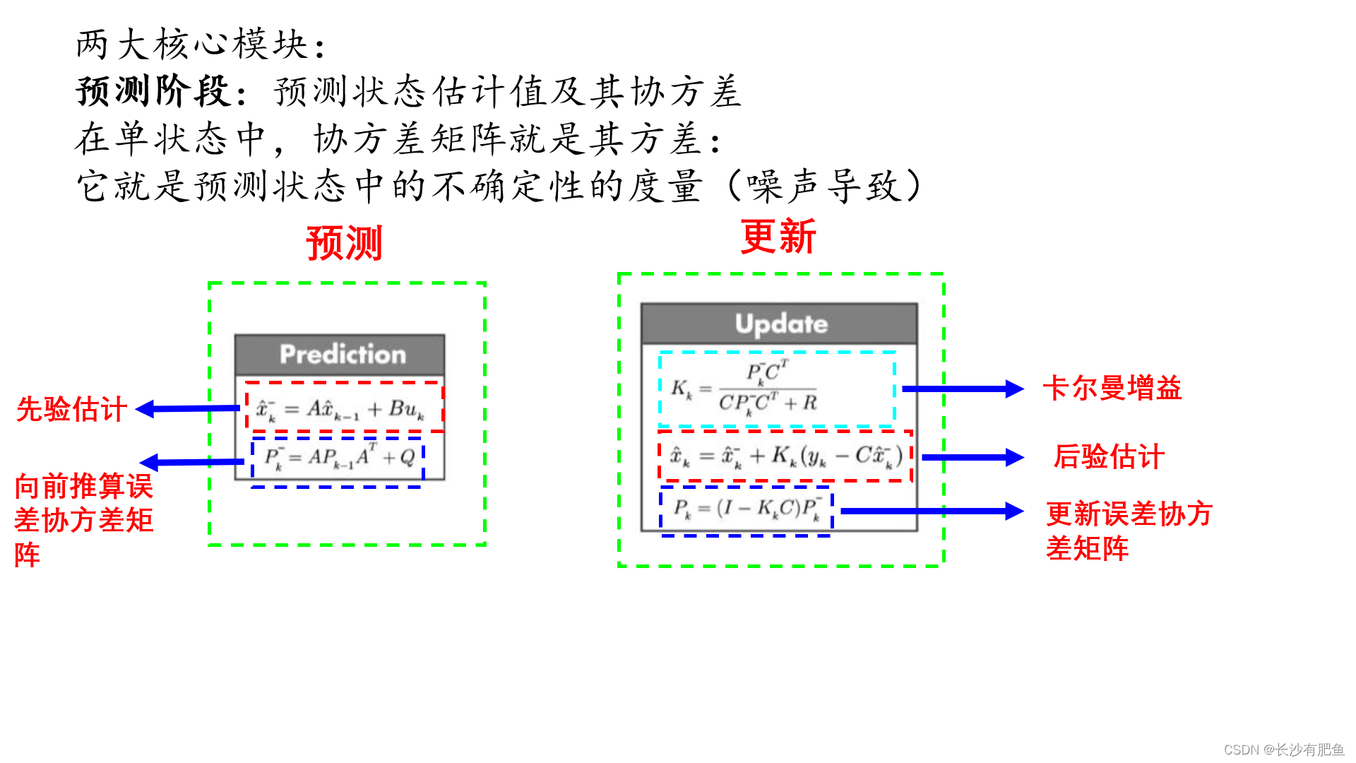
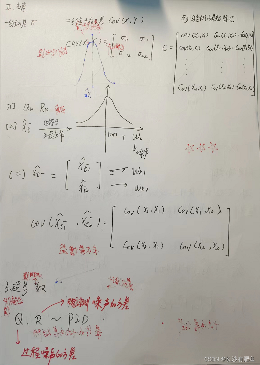
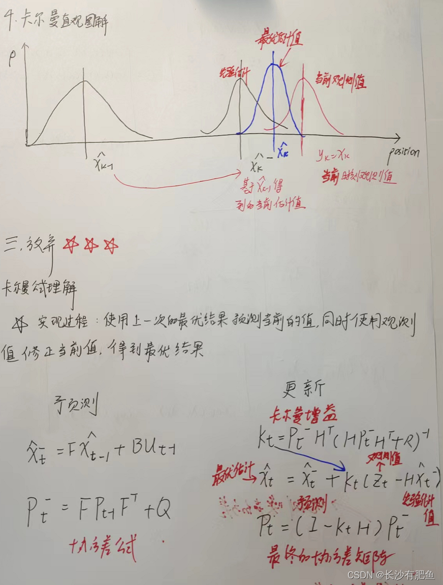
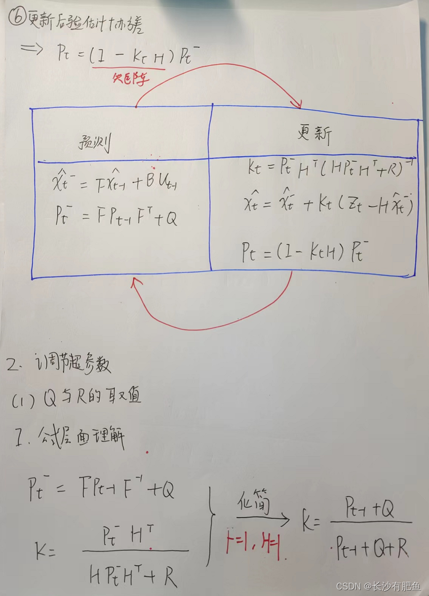
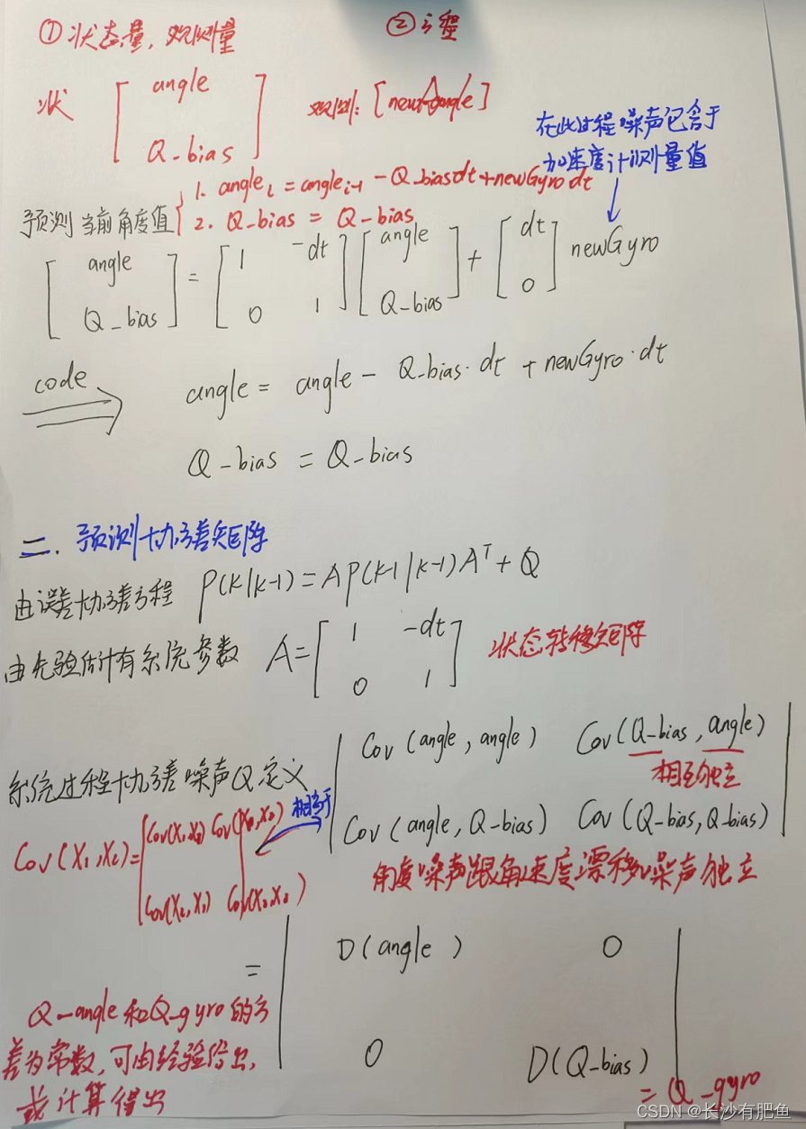
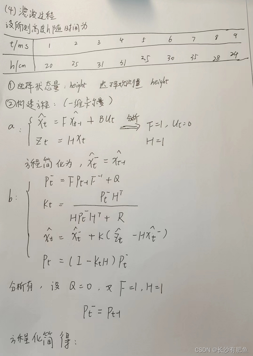
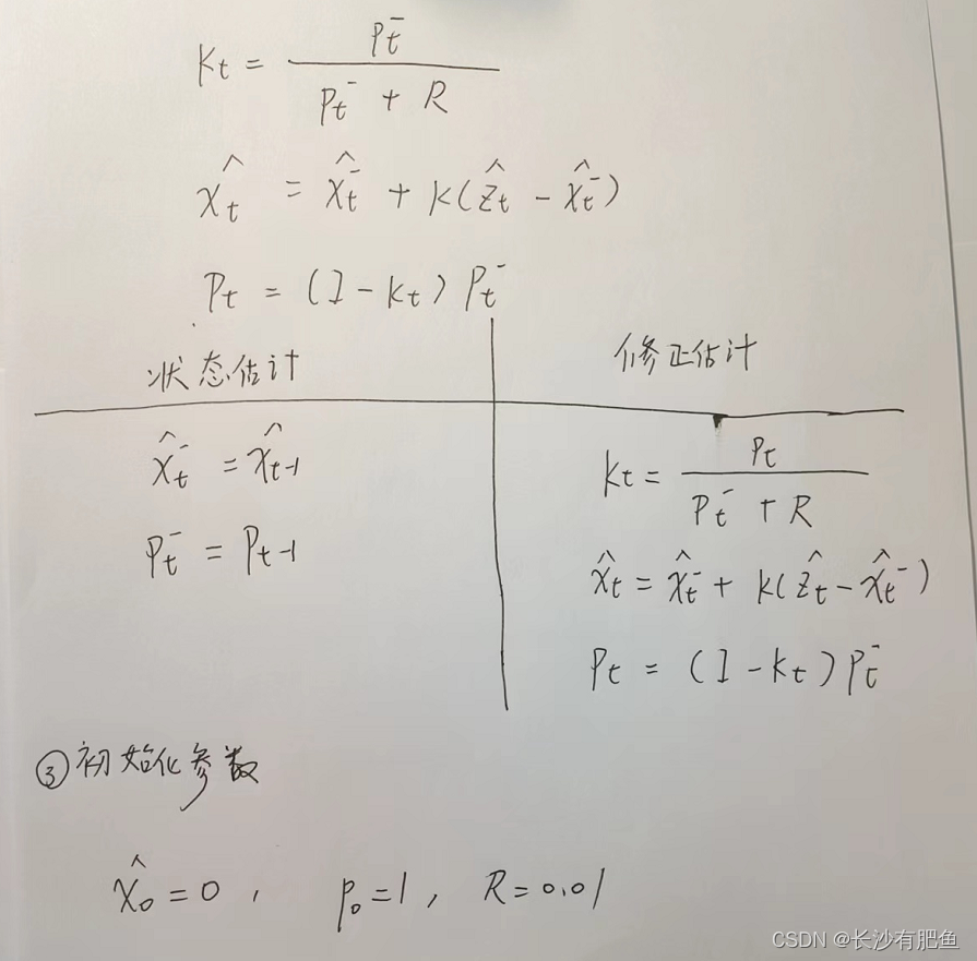
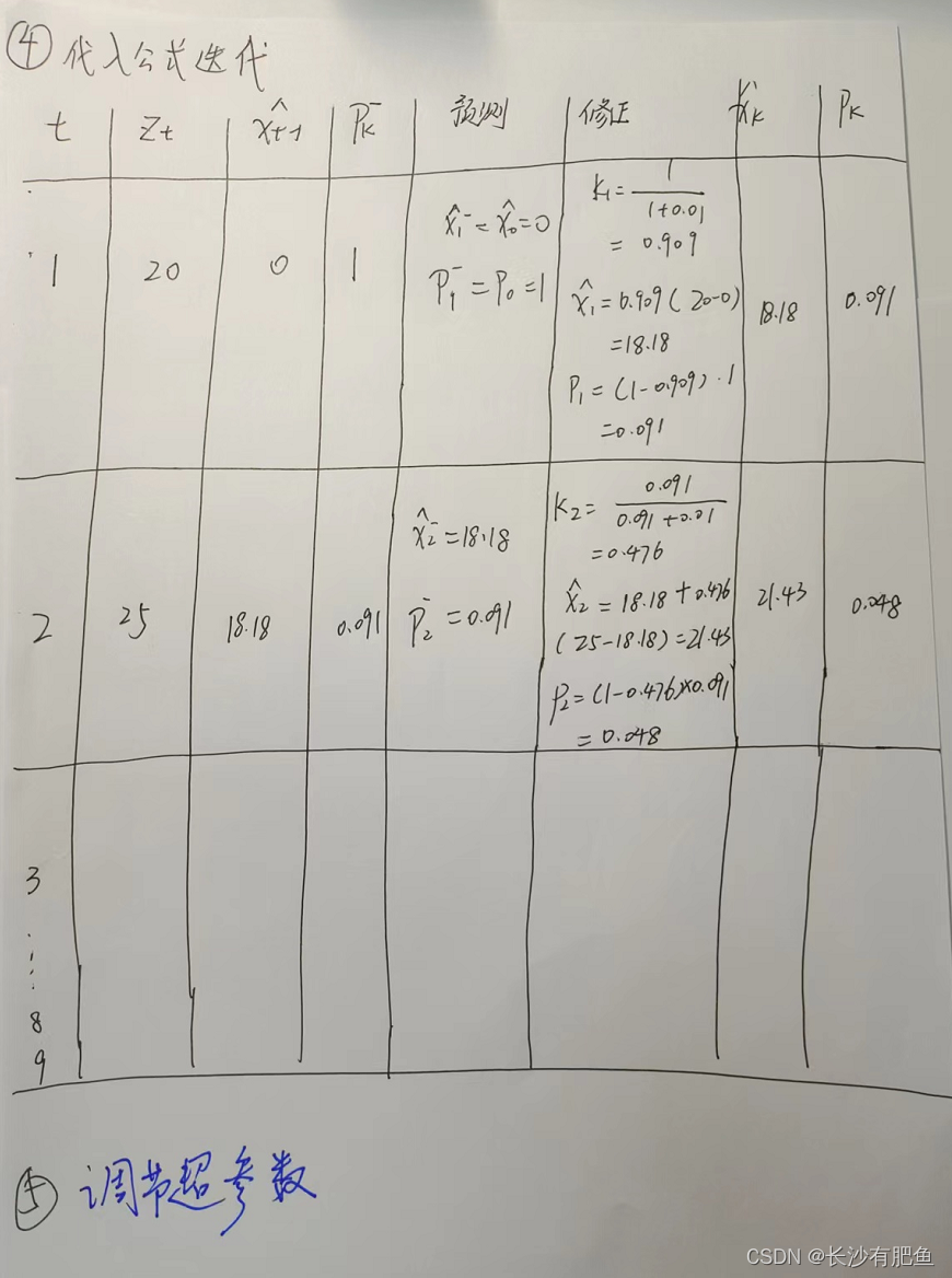
写在前面:卡尔曼滤波这一块比较晦涩难懂,通俗点讲,按我的理解就是利用已知信息去估计最优的位置,比如说,一个人或者一辆车下一时刻会在什么位置,卡尔曼滤波干的就是这个,利用相关的数学方法去算出下一个位置最可能在哪,其本质上是优化估计算法。
今天是6月7号,祝愿莘莘学子,金榜题名,今天高考的学生考上大学后,在查找资料时,这篇博客或许会被今天的一些学生看到,祝愿他们,愿他们青出于蓝而胜于蓝(因为我很菜),变成这方面的专家,到时候带带我!!
上面扯了这么多,大家如果看不清,可以从我的百度网盘里下载,文末有一些整理的代码,感兴趣的话,大家可以去研究一下!!
链接:https://pan.baidu.com/s/1MZNHKxtO3pgF6iWfp5pbyw
提取码:8888
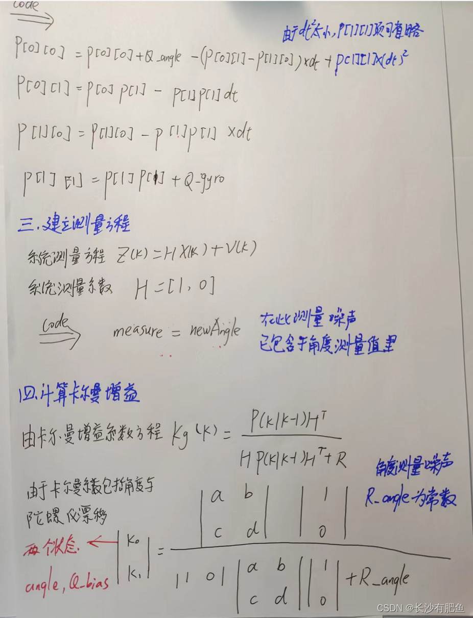
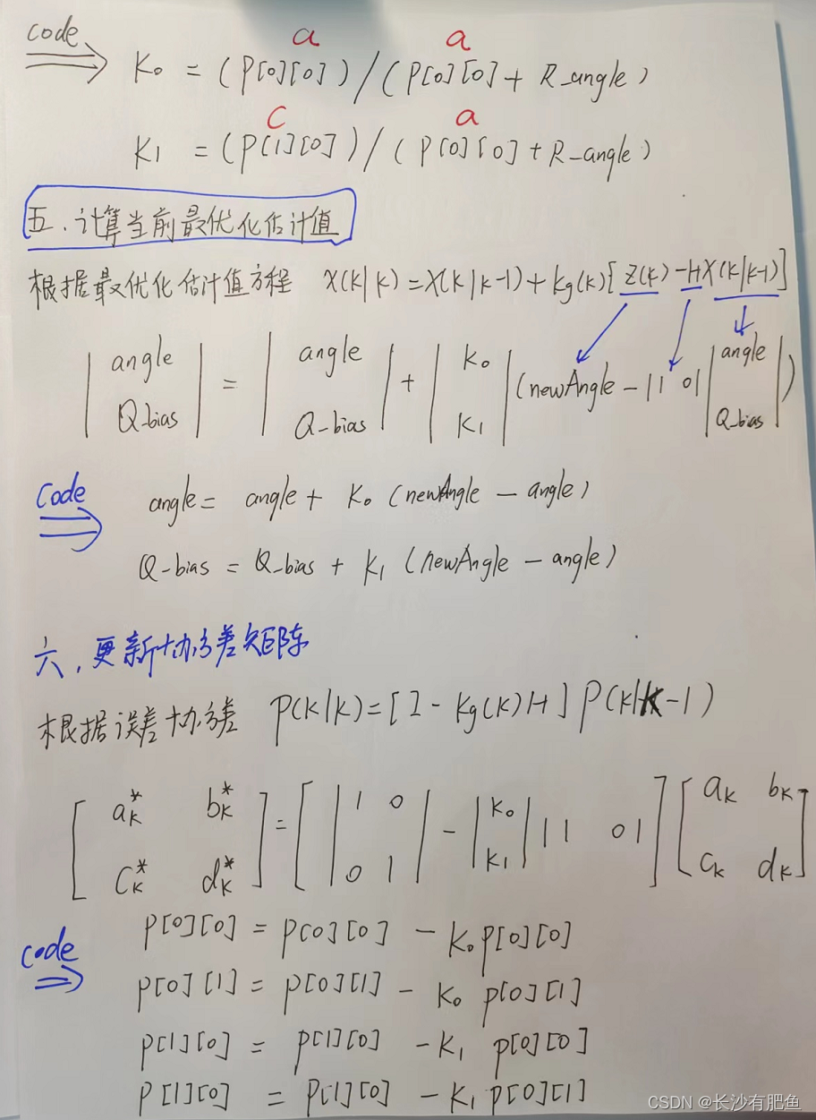
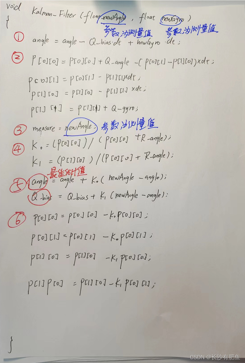
看了B站这位大神的讲解,自己手写了一份,讲的挺好的,大家可以去看看(感谢大佬的讲解)
从放弃到精通!卡尔曼滤波从理论到实践~_哔哩哔哩_bilibili

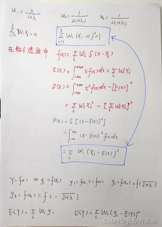
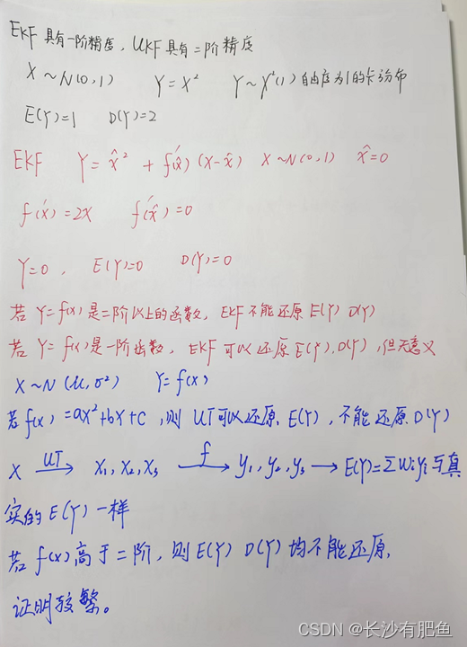
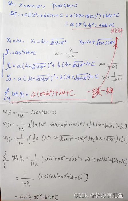
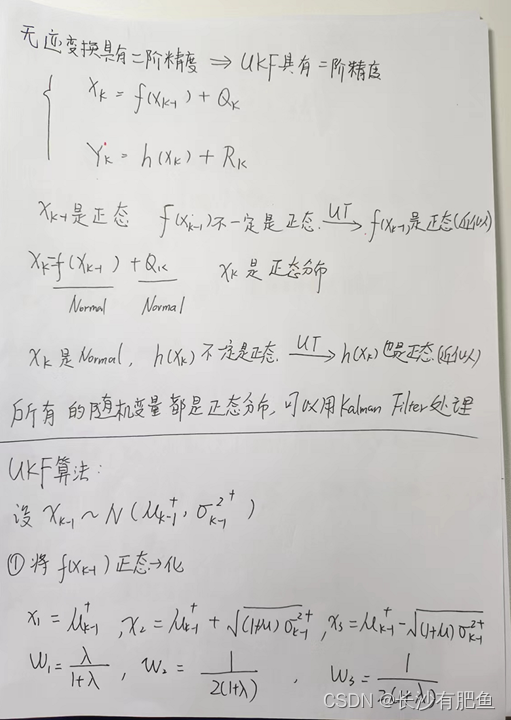
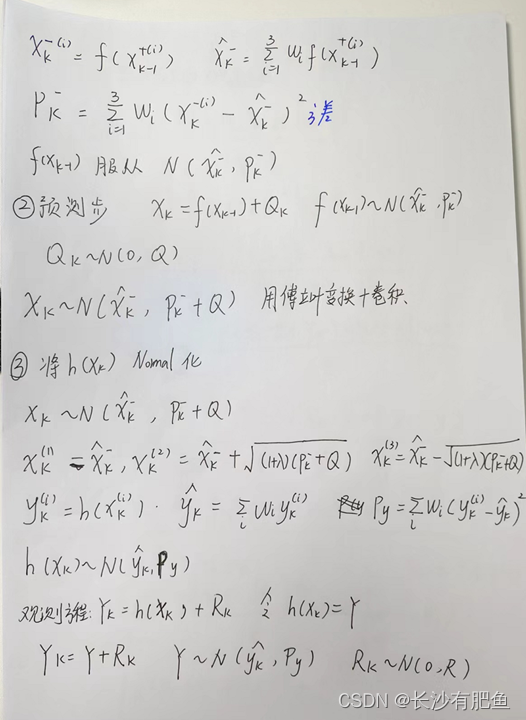
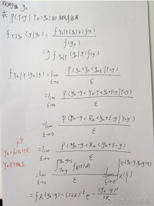
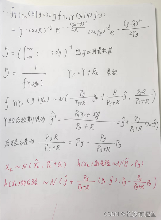
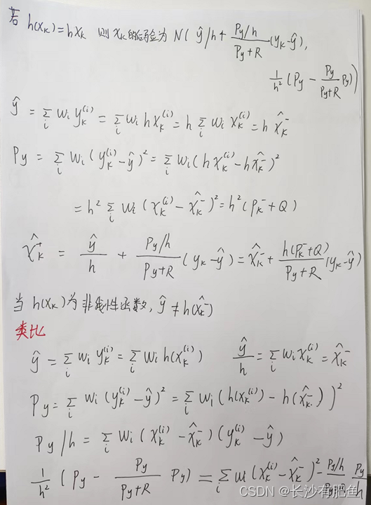
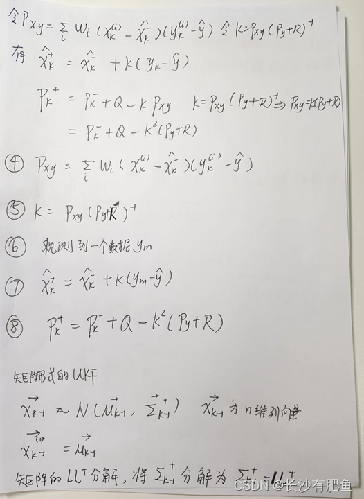
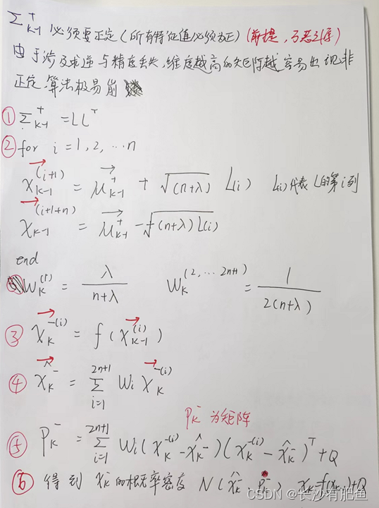
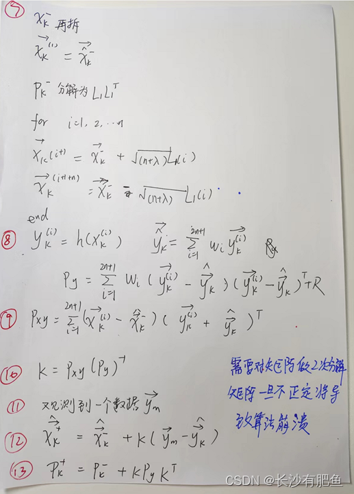
UKF推导:
贝叶斯滤波与卡尔曼滤波第十四讲 无迹卡尔曼滤波_哔哩哔哩_bilibili
感谢B站大佬的讲解,虽然手写了一遍,依旧看不懂(主要是我太菜),但是大佬很强,也很谦虚,非常感谢!!


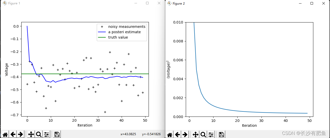
KF小例子:
# -*- coding=utf-8 -*-
# Kalman filter example demo in Python

# A Python implementation of the example given in pages 11-15 of "An
# Introduction to the Kalman Filter" by Greg Welch and Gary Bishop,
# University of North Carolina at Chapel Hill, Department of Computer
# Science, TR 95-041,

# coding:utf-8
import numpy
import pylab

# 这里是假设A=1,H=1的情况

# intial parameters
n_iter = 50
sz = (n_iter,) # size of array
x = -0.37727 # truth value (typo in example at top of p. 13 calls this z)
z = numpy.random.normal(x,0.1,size=sz) # observations (normal about x, sigma=0.1)

Q = 1e-5 # process variance

# allocate space for arrays
xhat=numpy.zeros(sz)      # a posteri estimate of x
P=numpy.zeros(sz)         # a posteri error estimate
xhatminus=numpy.zeros(sz) # a priori estimate of x
Pminus=numpy.zeros(sz)    # a priori error estimate
K=numpy.zeros(sz)         # gain or blending factor

R = 0.1**2 # estimate of measurement variance, change to see effect

# intial guesses
xhat[0] = 0.0
P[0] = 1.0

for k in range(1,n_iter):
    # time update
    xhatminus[k] = xhat[k-1]  #X(k|k-1) = AX(k-1|k-1) + BU(k) + W(k),A=1,BU(k) = 0
    Pminus[k] = P[k-1]+Q      #P(k|k-1) = AP(k-1|k-1)A' + Q(k) ,A=1

    # measurement update
    K[k] = Pminus[k]/( Pminus[k]+R ) #Kg(k)=P(k|k-1)H'/[HP(k|k-1)H' + R],H=1
    xhat[k] = xhatminus[k]+K[k]*(z[k]-xhatminus[k]) #X(k|k) = X(k|k-1) + Kg(k)[Z(k) - HX(k|k-1)], H=1
    P[k] = (1-K[k])*Pminus[k] #P(k|k) = (1 - Kg(k)H)P(k|k-1), H=1

pylab.figure()
pylab.plot(z,'k+',label='noisy measurements')     #测量值
pylab.plot(xhat,'b-',label='a posteri estimate')  #过滤后的值
pylab.axhline(x,color='g',label='truth value')    #系统值
pylab.legend()
pylab.xlabel('Iteration')
pylab.ylabel('Voltage')

pylab.figure()
valid_iter = range(1,n_iter) # Pminus not valid at step 0
pylab.plot(valid_iter,Pminus[valid_iter],label='a priori error estimate')
pylab.xlabel('Iteration')
pylab.ylabel('$(Voltage)^2$')
pylab.setp(pylab.gca(),'ylim',[0,.01])
pylab.show()
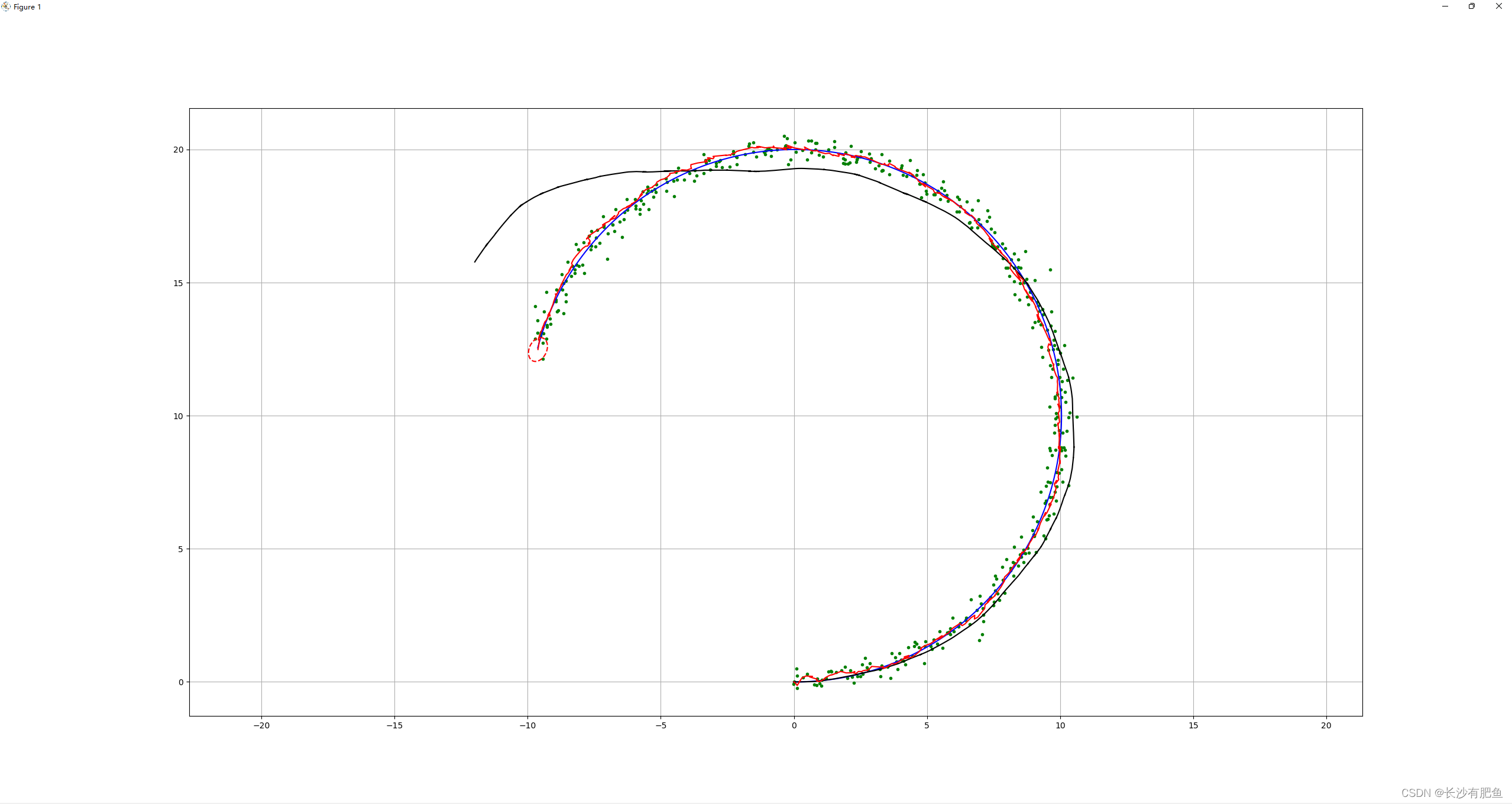
EKF小例子:
import numpy as np
import math
import matplotlib.pyplot as plt

# Estimation parameter of EKF
Q = np.diag([0.1, 0.1, np.deg2rad(1.0), 1.0])**2
R = np.diag([1.0, np.deg2rad(40.0)])**2

#  Simulation parameter
Qsim = np.diag([0.5, 0.5])**2
Rsim = np.diag([1.0, np.deg2rad(30.0)])**2

DT = 0.1  # time tick [s]
SIM_TIME = 50.0  # simulation time [s]

show_animation = True


def calc_input():
    v = 1.0  # [m/s]
    yawrate = 0.1  # [rad/s]
    u = np.matrix([v, yawrate]).T
    return u


def observation(xTrue, xd, u):

    xTrue = motion_model(xTrue, u)

    # add noise to gps x-y
    zx = xTrue[0, 0] + np.random.randn() * Qsim[0, 0]
    zy = xTrue[1, 0] + np.random.randn() * Qsim[1, 1]
    z = np.matrix([zx, zy])

    # add noise to input
    ud1 = u[0, 0] + np.random.randn() * Rsim[0, 0]
    ud2 = u[1, 0] + np.random.randn() * Rsim[1, 1]
    ud = np.matrix([ud1, ud2]).T

    xd = motion_model(xd, ud)

    return xTrue, z, xd, ud


def motion_model(x, u):

    F = np.matrix([[1.0, 0, 0, 0],
                   [0, 1.0, 0, 0],
                   [0, 0, 1.0, 0],
                   [0, 0, 0, 0]])

    B = np.matrix([[DT * math.cos(x[2, 0]), 0],
                   [DT * math.sin(x[2, 0]), 0],
                   [0.0, DT],
                   [1.0, 0.0]])

    x = F * x + B * u

    return x


def observation_model(x):
    #  Observation Model
    H = np.matrix([
        [1, 0, 0, 0],
        [0, 1, 0, 0]
    ])

    z = H * x

    return z


def jacobF(x, u):
    """
    Jacobian of Motion Model
    motion model
    x_{t+1} = x_t+v*dt*cos(yaw)
    y_{t+1} = y_t+v*dt*sin(yaw)
    yaw_{t+1} = yaw_t+omega*dt
    v_{t+1} = v{t}
    so
    dx/dyaw = -v*dt*sin(yaw)
    dx/dv = dt*cos(yaw)
    dy/dyaw = v*dt*cos(yaw)
    dy/dv = dt*sin(yaw)
    """
    yaw = x[2, 0]
    v = u[0, 0]
    jF = np.matrix([
        [1.0, 0.0, -DT * v * math.sin(yaw), DT * math.cos(yaw)],
        [0.0, 1.0, DT * v * math.cos(yaw), DT * math.sin(yaw)],
        [0.0, 0.0, 1.0, 0.0],
        [0.0, 0.0, 0.0, 1.0]])

    return jF


def jacobH(x):
    # Jacobian of Observation Model
    jH = np.matrix([
        [1, 0, 0, 0],
        [0, 1, 0, 0]
    ])

    return jH


def ekf_estimation(xEst, PEst, z, u):

    #  Predict
    xPred = motion_model(xEst, u)
    jF = jacobF(xPred, u)
    PPred = jF * PEst * jF.T + Q

    #  Update
    jH = jacobH(xPred)
    zPred = observation_model(xPred)
    y = z.T - zPred
    S = jH * PPred * jH.T + R
    K = PPred * jH.T * np.linalg.inv(S)
    xEst = xPred + K * y
    PEst = (np.eye(len(xEst)) - K * jH) * PPred

    return xEst, PEst


def plot_covariance_ellipse(xEst, PEst):
    Pxy = PEst[0:2, 0:2]
    eigval, eigvec = np.linalg.eig(Pxy)

    if eigval[0] >= eigval[1]:
        bigind = 0
        smallind = 1
    else:
        bigind = 1
        smallind = 0

    t = np.arange(0, 2 * math.pi + 0.1, 0.1)
    a = math.sqrt(eigval[bigind])
    b = math.sqrt(eigval[smallind])
    x = [a * math.cos(it) for it in t]
    y = [b * math.sin(it) for it in t]
    angle = math.atan2(eigvec[bigind, 1], eigvec[bigind, 0])
    R = np.matrix([[math.cos(angle), math.sin(angle)],
                   [-math.sin(angle), math.cos(angle)]])
    fx = R * np.matrix([x, y])
    px = np.array(fx[0, :] + xEst[0, 0]).flatten()
    py = np.array(fx[1, :] + xEst[1, 0]).flatten()
    plt.plot(px, py, "--r")


def main():
    print(__file__ + " start!!")

    time = 0.0

    # State Vector [x y yaw v]'
    xEst = np.matrix(np.zeros((4, 1)))
    xTrue = np.matrix(np.zeros((4, 1)))
    PEst = np.eye(4)

    xDR = np.matrix(np.zeros((4, 1)))  # Dead reckoning

    # history
    hxEst = xEst
    hxTrue = xTrue
    hxDR = xTrue
    hz = np.zeros((1, 2))

    while SIM_TIME >= time:
        time += DT
        u = calc_input()

        xTrue, z, xDR, ud = observation(xTrue, xDR, u)

        xEst, PEst = ekf_estimation(xEst, PEst, z, ud)

        # store data history
        hxEst = np.hstack((hxEst, xEst))
        hxDR = np.hstack((hxDR, xDR))
        hxTrue = np.hstack((hxTrue, xTrue))
        hz = np.vstack((hz, z))

        if show_animation:
            plt.cla()
            plt.plot(hz[:, 0], hz[:, 1], ".g")
            plt.plot(np.array(hxTrue[0, :]).flatten(),
                     np.array(hxTrue[1, :]).flatten(), "-b")
            plt.plot(np.array(hxDR[0, :]).flatten(),
                     np.array(hxDR[1, :]).flatten(), "-k")
            plt.plot(np.array(hxEst[0, :]).flatten(),
                     np.array(hxEst[1, :]).flatten(), "-r")
            plot_covariance_ellipse(xEst, PEst)
            plt.axis("equal")
            plt.grid(True)
            plt.pause(0.001)


if __name__ == '__main__':
    main()
最后整理了一些代码,有需要的可以自己下载去看看,哪些可以用到,卡尔曼滤波的博大精深不是一时半会就搞定的,哎,真的好难呀,希望大家多多指教!!
链接:https://pan.baidu.com/s/1aeyGpRS5uqHq4U2NAqdh5w
提取码:8888


 3万+
3万+


 被折叠的 条评论
为什么被折叠?
被折叠的 条评论
为什么被折叠?
 到【灌水乐园】发言


