


**论文信息:**Deep Clustering via Joint Convolutional Autoencoder Embedding and Relative Entropy Minimization
基于联合卷积自编码器嵌入和相对熵最小化的深度聚类
[1704.06327] Deep Clustering via Joint Convolutional Autoencoder Embedding and Relative Entropy Minimization
2017年发表于ML
摘要
论文提出了一个新的聚类模型—Deep Embedded RegularIzed ClusTering (DEPICT),最大的亮点是DEPICT将卷积自编码器应用于聚类任务,它可以有效的学习具有辨别性的嵌入子空间并且进行精准的聚类分配。
1)为了解决图像聚类遇到的特征提取质量差的问题,DEPICT最先在无监督聚类任务上使用了卷积和反卷积构造卷积自编码器。2)为了提升训练效率,DEPICT不像DEC那样进行预训练,而是引入了一个联合学习框架来最小化统一的聚类和重建损失函数,并同时训练所有的网络层。3)此外,使用自编码器中的重构损失函数,作为一个数据相关的正则化项,以防止深度嵌入函数的过拟合。
实验结果表明,在没有标记数据(无监督)可用于超参数调优的现实聚类任务中,DEPICT算法具有优势和更快的运行时间。
Abstract
This week’s I read Deep Clustering via Joint Convolutional Autoencoder Embedding and Relative Entropy Minimization, which introduces DEPICT, a novel deep clustering model. DEPICT leverages convolutional autoencoders to learn discriminative embeddings for clustering tasks. It employs a joint learning framework that minimizes a unified loss function combining clustering and reconstruction losses, eliminating the need for pretraining. The model incorporates a regularization term to balance cluster frequencies and uses a noisy encoder to ensure robustness against input noise. Experimental results on the MNIST dataset demonstrate DEPICT’s superior clustering accuracy and efficiency compared to previous methods like DEC. The report concludes by discussing the potential for exploring different encoder architectures for clustering tasks beyond image data.
卷积自编码器
卷积自编码器通常设计成全卷积神经网络的结构,最早使用CNN构建卷积自编码器的是 Stacked Convolutional Auto-Encoders for Hierarchical Feature Extraction https://link.springer.com/chapter/10.1007/978-3-642-21735-7_7
但是此文中作者提出的CAE是为了用作预训练,预训练后将权重用于CNN进行有监督的分类任务。
Joint Unsupervised Learning of Deep Representations and Image Clusters [1604.03628] Joint Unsupervised Learning of Deep Representations and Image Clusters 中提出了用于聚类的JULE模型,JULE最先将CNN用于聚类任务中,精心构造了一个损失函数用于计算聚类和实际损失,并使用这个损失函数进行联合训练。但是实际上他们只构建了一个编码器结构,并非一个完整的自编码器,而且依赖于标签数据所以并非完全的无监督过程。
DEPICT受到启发,构造一个完整的卷积自编码器,并将编码器输出的特征的聚类损失,加上整个自编码器的重建损失,统一损失进行联合训练。
DEPICT
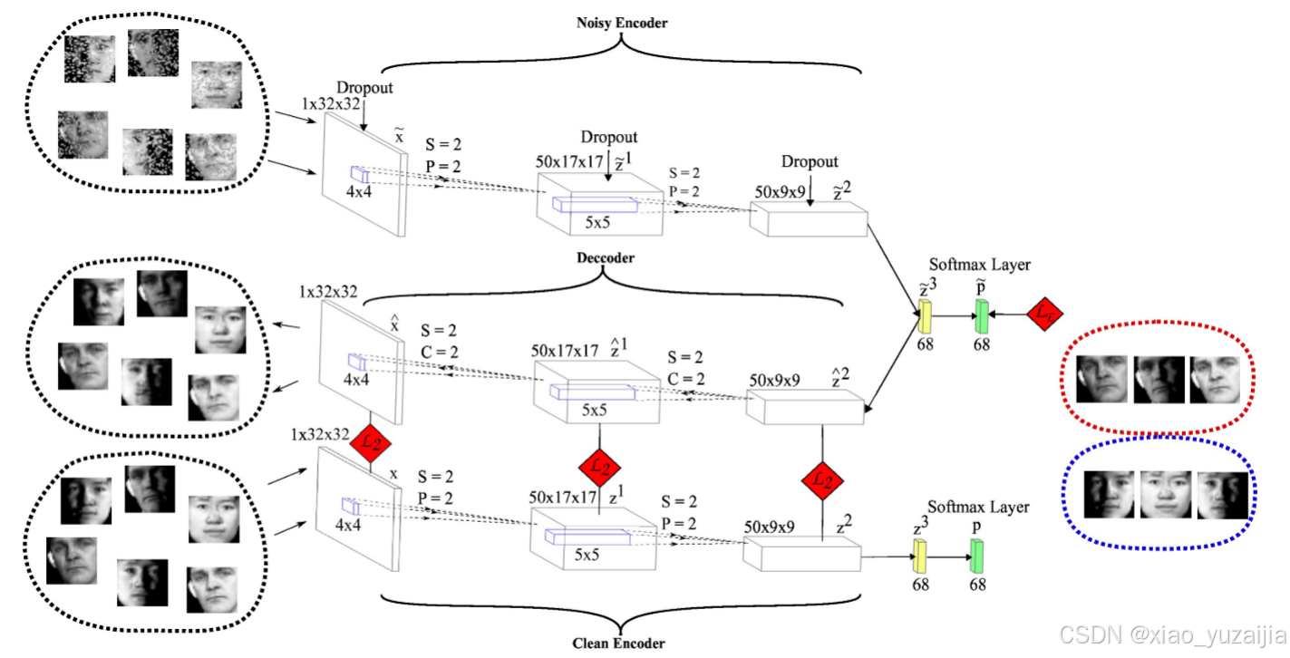
CMU-PIE数据集的DEPICT架构。DEPICT由堆叠在多层卷积自编码器上的软最大层组成。为了说明联合学习框架,我们考虑了以下四种DEPICT途径:噪声(rdopout)编码器,解码器,干净编码器和Soft-max层。聚类损失函数L_E应用于噪声路径,重建损失函数L_2位于解码器层和干净编码器层之间。卷积层的输出大小、核大小、步幅(S)、填充§和作物©也在图中显示。
聚类损失
和所有的自编码结构模型一样,将原始样本表示 X X X通过嵌入函数得到低维的表示 Z Z Z。给定学习到的嵌入特征,使用多项式逻辑回归(soft-max)函数 f θ : Z − > Y f_θ: Z ->Y fθ:Z−>Y预测聚类分配的概率P。

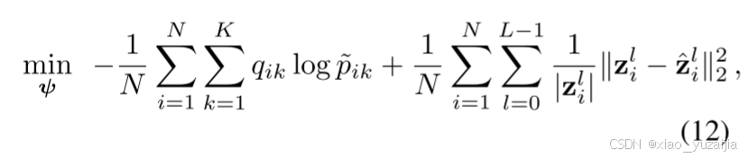
为了定义聚类目标函数,使用辅助目标变量Q迭代细化模型预测P。因为P和Q显然都是样本到类簇的一个概率状况,因此可以理解为分布概率。为此,作者首先使用KL散度来减少模型预测P与目标变量Q之间的距离。(这一点与DEC中使用是一致的)

为了避免 “退化解” 将大部分样本分配给几个簇或分配给离群样本,作者采用了对目标变量施加一个正则化项以达到缓解或类簇平衡的目的。为此,首先将目标变量的经验标签分布定义为:

其中, f k f_k fk可以被认为是目标分布中聚类分配的软频率。使用这种经验分布,能够通过在损失函数中添加另一个KL散度来加强模型对平衡分配的偏好。

其中,u是经验标签分布的均匀先验。
目标函数中的第一项使目标和模型预测分布之间的距离最小化,而第二项平衡了目标变量中簇的频率。利用平衡的目标变量,我们可以间接地迫使模型有更平衡的预测(聚类分配)P。并且作者在这里指出,如果对簇的频率有任何额外的了解,那么将先验从均匀分布更改为目标函数中的任意分布也很简单。
论文中使用Clean feedforward (encoder) pathway计算目标变量Q,并通过Corrupted (noisy) feedforward (encoder) pathway建立模型预测 P ~ \tilde{P} P~。因此,聚类损失函数 K L ( Q ∣ ∣ P ~ ) KL(Q||\tilde{P}) KL(Q∣∣P~)迫使模型具有关于噪声的不变特征。换句话说,模型被假设具有双重作用:使用Clean feedforward (encoder)计算更准确的目标变量;Corrupted (noisy) feedforward (encoder),经过训练以实现噪声不变预测。
重构损失
重构损失来自于编码器与解码器各个对应的层与层之间,使用均方根误差。
将聚类损失与重构损失相加得到总损失,利用这个损失进行联合学习。
结果
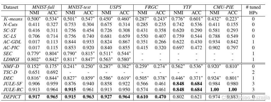
仅从MNIST数据上看,DEPICT就已经比DEC还高,在测试集上做到了96.3%的准确率。
实验
DEPICT的pytorch实现,以MNIST数据集为例。项目地址github.com
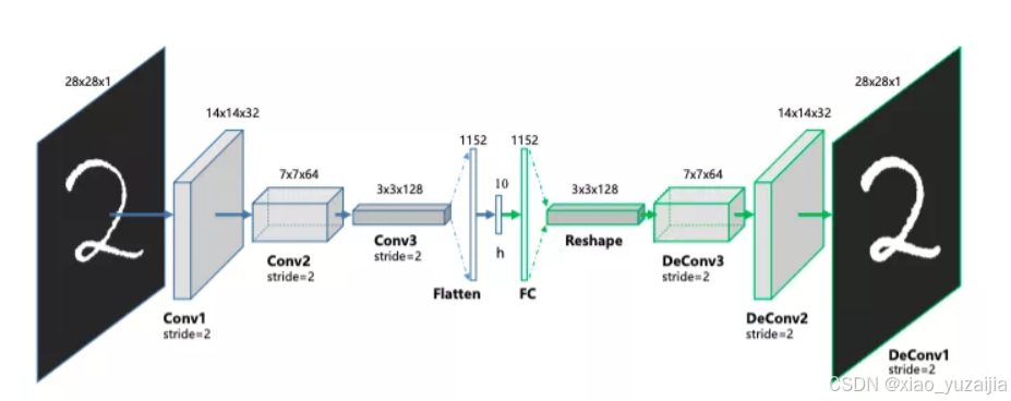
网络结构
整个卷积自编码器网络的特征图结构为[28x28, 28x28, 28x28, 28x28,14x14, 28x28, 28x28, 28x28, 28x28]。
通道数结构为[1, 64, 64, 1, 1, 1, 64, 64, 1]
注意还有一层线性层和softmax层,不过这两层只用于聚类和聚类损失
class autoencoder(nn.Module):
  def __init__(self,n_clus):
    super(autoencoder,self).__init__()
    self.encoder1 = nn.Sequential(
                nn.Conv2d(1,64,kernel_size=3,stride=1,padding=1),
                nn.BatchNorm2d(64),
                nn.Sigmoid())
    self.encoder2 =  nn.Sequential(
                nn.Conv2d(64,64,kernel_size=3,stride=1,padding=1),
                nn.BatchNorm2d(64),
                nn.Sigmoid())
    self.encoder3 =  nn.Sequential(
                nn.Conv2d(64,1,kernel_size=3,stride=1,padding=1),
                nn.BatchNorm2d(1),
                nn.Sigmoid())
    self.encoder4 = nn.Sequential(
                nn.Conv2d(1,1,kernel_size=2,stride=2,padding=0),
                nn.BatchNorm2d(1),
                nn.Sigmoid())
    self.decoder4 = nn.Sequential(
                nn.ConvTranspose2d(1,1,kernel_size=2,stride=2,padding=0),
                nn.BatchNorm2d(1),
                nn.Sigmoid())
    self.decoder3 = nn.Sequential(
                nn.Conv2d(1,64,kernel_size=3,stride=1,padding=1),
                nn.BatchNorm2d(64),
                nn.Sigmoid()
                )
    self.decoder2 =  nn.Sequential(
                nn.Conv2d(64,64,kernel_size=3,stride=1,padding=1),
                nn.BatchNorm2d(64),
                nn.Sigmoid())
    self.decoder1 = nn.Sequential(
                nn.Conv2d(64,1,kernel_size=3,stride=1,padding=1),
                nn.BatchNorm2d(1),
                nn.Sigmoid())
    self.n_clus = n_clus
    self.em = nn.Linear(14*14,self.n_clus)
  def forward(self,x):
    enc1 = self.encoder1(x)
    enc2 = self.encoder2(enc1)
    enc3 = self.encoder3(enc2)
    enc4 = self.encoder4(enc3)
    dec4 = self.decoder4(enc4)
    dec3 = self.decoder3(dec4)
    dec2 = self.decoder2(dec3)
    dec1 = self.decoder1(dec2)
    x = enc4.view(-1, 14*14)
    em = self.em(x)
    em = F.softmax(em, dim=1)
    return (enc1,enc2,enc3,enc4,dec4,dec3,dec2,dec1,em)
  def obtain_batch_loss(self,x,beta):
    enc1,enc2,enc3,enc4,dec4,dec3,dec2,dec1,em=self.forward(x)
    loss1 = nn.BCELoss()(dec1,x)
    loss2 = nn.MSELoss()(dec2,enc1)
    loss3 = nn.MSELoss()(dec3,enc2)
    loss4 = nn.MSELoss()(dec4,enc3)
    r_sumoveri = torch.sqrt(torch.sum(em,dim=0))
    num = em/r_sumoveri
    q = num/(torch.sum(num,dim=0))
    clus_loss = -1*torch.mean(q*torch.log(em))/self.n_clus  # 聚类损失
    recons_loss = loss1+beta*(loss2+loss3+loss4)  # 重构损失
    return (clus_loss,recons_loss)
  def encode(self,x):
    enc1 = self.encoder1(x)
    enc2 = self.encoder2(enc1)
    enc3 = self.encoder3(enc2)
    enc4 = self.encoder4(enc3)
    return enc4
训练
重点理解一下损失计算。
聚类损失:首先计算目标分布Q,真实分布P则由编码器通过线性层和softmax层获得,最后根据公式得到聚类损失。
重构损失:重构损失来自于编码器与解码器各个对应的层与层之间,使用均方根误差。
聚类损失和重构损失相加得到联合损失。
for epoch in range(epochs):
    minloss = 1
    running_clus_loss=0
    running_recons_loss=0
    num_images=0
    for i,(img,_) in enumerate(train_loader):
      img = img.to(device)
      optim.zero_grad()
      clus_loss,recons_loss = autoenc.obtain_batch_loss(img,0.8)
      loss=recons_loss+clus_loss
      loss.backward()
      optim.step()
      running_clus_loss = running_clus_loss + clus_loss.item()*len(img)
      running_recons_loss = running_recons_loss + recons_loss.item()*len(img)
      num_images= num_images+len(img)
    print('epoch: '+str(epoch)+' clus_loss: '+str(running_clus_loss/num_images)+' recons_loss: '+str(running_recons_loss/num_images))
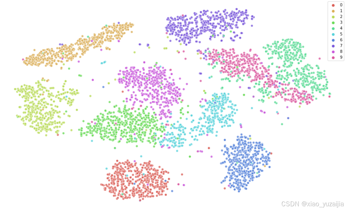
结果
使用T-SNE对特征进行可视化,可以发现分类效果良好。
总结
DEPICT通过卷积自编码器和联合训练的方式,将聚类准确率又提升到了一个新高度,而且聚类损失中的第二项KL散度正则化也相当有趣。但是卷积自编码器在图像数据上具有天然优势,在其他数据上的效果可能就比较平庸。未来可以探索其他的编码器结构在文本等其他数据聚类上的研究。


 721
721

 被折叠的 条评论
为什么被折叠?
被折叠的 条评论
为什么被折叠?
 到【灌水乐园】发言


